Boundary Conditions
Nonreflecting Boundaries
The modeling of geomechanics problems involves media which, at the scale of the analysis, are better represented as unbounded. Deep underground excavations are normally assumed to be surrounded by an infinite medium, while surface and near-surface structures are assumed to lie on a half-space. Numerical methods relying on the discretization of a finite region of space require that appropriate conditions be enforced at the artificial numerical boundaries. In static analyses, fixed or elastic boundaries (e.g., represented by boundary element techniques) can be realistically placed at some distance from the region of interest. In dynamic problems, however, such boundary conditions cause the reflection of outward propagating waves back into the model, and do not allow the necessary energy radiation. The use of a larger model can minimize the problem, since material damping will absorb most of the energy in the waves reflected from distant boundaries. However, this solution leads to large computational costs. The alternative is to use nonreflecting (or absorbing) boundaries. Several formulations have been proposed. The viscous boundary developed by Lysmer and Kuhlemeyer (1969) is used in 3DEC. It is based on the use of independent dashpots, and is nearly totally effective for body waves approaching the boundary at angles of incidence above 30°. For lower angles of incidence, or for surface waves, the energy absorption is only approximate. However, it has the advantage of being an effective technique which can be used in time-domain analyses. Its effectiveness has been demonstrated in both finite-element and finite-difference models (Kunar et al. 1977). A variation of this technique proposed by White et al. (1977) is also widely used.
More efficient energy absorption (for example, in the case of Rayleigh waves) requires the use of frequency-dependent dashpots, which can only be used in frequency-domain analyses (e.g., Lysmer and Waas 1972). These are usually designated as consistent boundaries, and involve the calculation of dynamic-stiffness matrices coupling all the boundary degrees-of-freedom. Boundary-element methods may be used to derive these matrices (e.g., Wolf 1985). A comparative study of the performance of different types of elementary, viscous and consistent boundaries was reported by Roesset and Ettouney (1977).
A different procedure to obtain efficient absorbing boundaries for use in time-domain studies was proposed by Cundall et al. (1978). It is based on the superposition of solutions with stress and velocity boundaries in such a way that reflections are canceled. In practice, it requires adding the results of two parallel, overlapping grids in a narrow region adjacent to the boundary. This method has been shown to provide effective energy absorption, but is difficult to implement for a blocky system with complex geometry, and thus, is not used in 3DEC.
The viscous boundaries proposed by Lysmer and Kuhlemeyer (1969) consist of independent dashpots attached to the boundary in the normal and shear directions. They provide viscous normal and shear tractions given by
where:
\(v_n\) and \(v_s\) are the normal and shear components of the velocity at the boundary;
\(\rho\) is the mass density; and
\(C_p\) and \(C_s\) are the \(p\)- and \(s\)-wave velocities.
These viscous terms can be introduced directly into the equations of motion of the gridpoints lying on the boundary. A different approach, however, was implemented in 3DEC, in which the tractions \(t_n\) and \(t_s\) are calculated and applied at every timestep in the same way as the boundary loads. This alternative scheme allows the viscous boundaries to be used with rigid blocks as well. Tests have shown that this implementation is equally effective. The only potential problem concerns numerical stability, because the viscous forces are calculated from velocities lagging by half a timestep. In practical analyses to date, no reduction of timestep has been required by the use of the nonreflecting boundaries. Timestep restrictions demanded by high joint stiffnesses or small zones are usually more important.
Dynamic analysis starts from some in-situ condition. If a velocity is used to provide the static stress state, this boundary condition can be replaced by nonreflecting boundaries; the boundary reaction forces should be maintained throughout the dynamic loading phase. If a stress boundary condition is applied for the static in-situ solution, a stress boundary condition of opposite sign must also be applied over the same boundary when the nonreflecting boundary is applied for the dynamic phase. This will allow the correct reaction forces to be in place at the boundary for the dynamic calculation.
Free-Field Boundaries
Numerical analysis of the seismic response of surface structures such as dams requires the discretization of a region of the material adjacent to the foundation. The seismic input is normally represented by plane waves propagating upward through the underlying material. The boundary conditions at the sides of the model must account for the free-field motion that would exist in the absence of the structure. In some cases, elementary lateral boundaries may be sufficient. For example, if only a shear wave were applied on the horizontal boundary AC, shown in Figure 1, it would be possible to fix the boundary along AB and CD in the vertical direction only. These boundaries should be placed at sufficient distances to minimize wave reflections and achieve free-field conditions. For soils with high material-damping, this condition can be obtained with a relatively small distance (Seed et al. 1975). However, when the material damping is low, the required distance may lead to an impractical model. An alternative procedure is to “enforce” the free-field motion in such a way that boundaries retain their nonreflecting properties (i.e., outward waves originating from the structure are properly absorbed). This approach was used in the continuum finite-difference code NESSI (Cundall et al. 1980). A technique of this type, involving the execution of free-field calculations in parallel with the main-grid analysis, was developed for 3DEC.
The lateral boundaries of the main grid are coupled to the free-field grid by viscous dashpots to simulate a quiet boundary (see Figure 1); the unbalanced forces from the free-field grid are applied to the main-grid boundary. Both conditions are expressed in following three equations, which apply to the free-field boundary along one side boundary plane with its normal in the direction of the \(x\)-axis. Similar expressions may be written for the other sides and corner boundaries:
where
\(\rho\) = density of material along vertical model boundary;
\(C_p\) = \(p\)-wave speed at the side boundary;
\(C_s\) = \(s\)-wave speed at the side boundary;
\(A\) = area of influence of free-field gridpoint;
\(v_x^m\) = \(x\)-velocity of gridpoint in main grid at side boundary;
\(v_y^m\) = \(y\)-velocity of gridpoint in main grid at side boundary;
\(v_z^m\) = \(z\)-velocity of gridpoint in main grid at side boundary;
\(v_x^{ff}\) = \(x\)-velocity of gridpoint in side free field;
\(v_y^{ff}\) = \(y\)-velocity of gridpoint in side free field;
\(v_z^{ff}\) = \(z\)-velocity of gridpoint in side free field;
\(F_x^{ff}\) = free-field gridpoint force with contributions from the \(\sigma_{xx}^{\rm ff}\) stresses of the free-field zones around the gridpoint;
\(F_y^{ff}\) = free-field gridpoint force with contributions from the \(\sigma_{xy}^{\rm ff}\) stresses of the free-field zones around the gridpoint; and
\(F_z^{ff}\) = free-field gridpoint force with contributions from the \(\sigma_{xz}^{\rm ff}\) stresses of the free-field zones around the gridpoint.
In this way, plane waves propagating upward suffer no distortion at the boundary because the freefield grid supplies conditions that are identical to those in an infinite model. If the main grid is uniform and there is no surface structure, the lateral dashpots are not exercised because the free-field grid executes the same motion as the main grid. However, if the main-grid motion differs from that of the free field (due, for example, to a surface structure that radiates secondary waves), then the dashpots act to absorb energy in a manner similar to quiet boundaries.
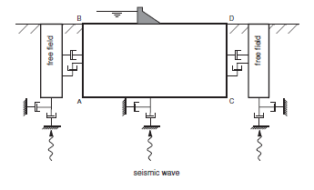
Figure 1: Model for seismic analysis of surface structures and free-field mesh.
In order to apply the free-field boundary in 3DEC, the model must be oriented such that the base is horizontal and its normal is in the direction of the \(y\)-axis, and the sides are vertical and their normals are in the direction of either the \(x\)- or \(z\)-axis. If the direction of propagation of the incident seismic waves is not vertical, then the coordinate axes can be rotated such that the \(y\)-axis coincides with the direction of propagation. In this case, gravity will act at an angle to the \(y\)-axis, and a horizontal free surface will be inclined with respect to the model boundaries.
The free-field model consists of four plane free-field grids, on the side boundaries of the model and four column free-field grids at the corners. The plane grids are generated to match the main-grid zones on the side boundaries, so that there is a one-to-one correspondence between gridpoints in the free field and the main grid. The four corner free-field columns act as free-field boundaries for the plane free-field grids. The plane free-field grids are two-dimensional calculations that assume infinite extension in the direction normal to the plane. The column free-field grids are one-dimensional calculations that assume infinite extension in both horizontal directions. Both the plane and column grids consist of standard 3DEC zones, which have gridpoints constrained in such a way to achieve the infinite extension assumption.
The model should be in static equilibrium before the free-field boundary is applied. The static equilibrium conditions prior to the dynamic analysis are transferred to the free field automatically when the command block dynamic free-field apply is invoked. The free-field condition is applied to lateral boundary gridpoints. All zone data (including model types and current state variables) in the model zones adjacent to the free field are copied to the free-field region. Free-field stresses are assigned the average stress of the neighboring grid zone. The dynamic boundary conditions at the base of the model should be specified before applying the free-field. These base conditions are automatically transferred to the free field when the free field is applied. Note that the free field is continuous; if the main grid contains an interface that extends to a model boundary, the interface will not continue into the free field.
After the block dynamic free-field apply command is issued, the free-field grid will plot automatically whenever blocks are plotted. Free-field information can be printed with the block dynamic free-field list command.
Example Using Dynamic Free Field
A simple model of a concrete gravity dam is created. The top boundary of the model is a free boundary. The base of the model is a viscous (quiet) boundary. Figure 2 shows the geometry of the model with the dam in the center on top. The model is initially run to static equilibrium under gravity, to equilibrate the body forces and the boundary forces. This must be done prior to applying the free field boundaries.
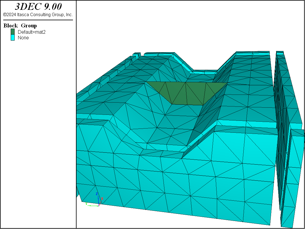
Figure 2: Model of dam with free field blocks visible.
The next step is to run the model with only viscous boundaries. An impulse shear stress function is applied to the base of the model. In this model, the boundaries are too close and it can be seen in Figure 3 that there is amplification of the \(x\)-velocities at the base, and distortion of the motion at the dam crest.
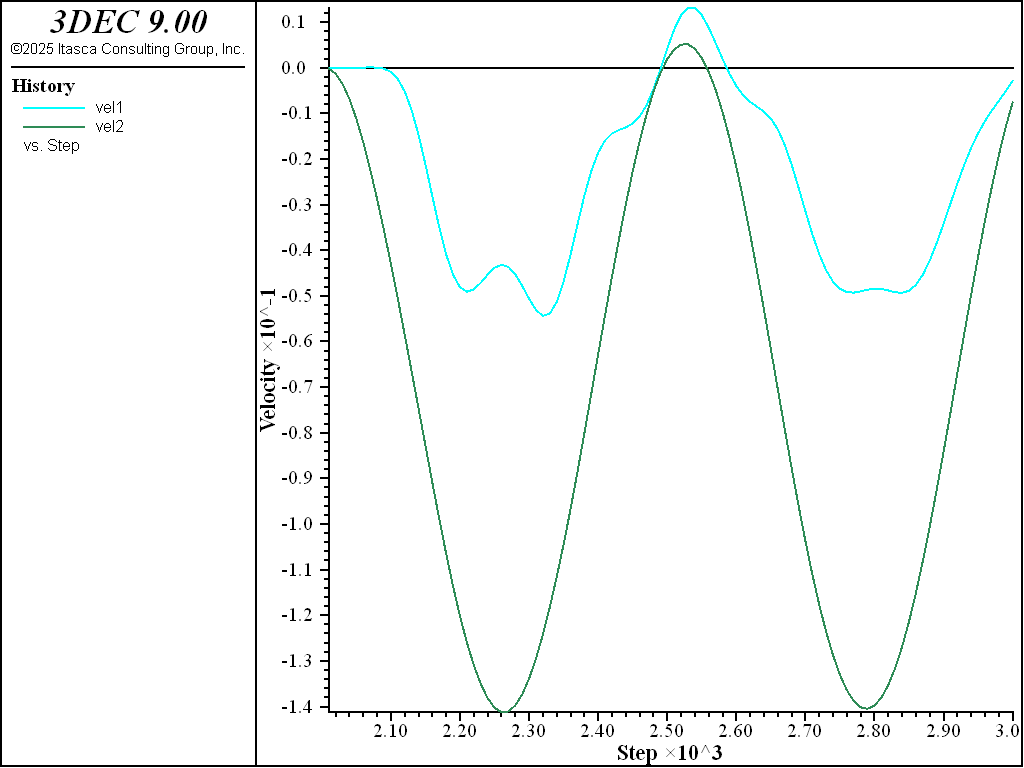
Figure 3: \(x\)-velocity histories at model base and dam crest using viscous boundaries.
Next, the model is rerun using the free field. The free field command creates new blocks at the boundary of the model and automatically zones them. Again, the impulse shear stress is applied to the base. The dynamic input consists of a sinusoidal shear stress wave applied at the model base. Figure 4 shows the \(x\)-velocity histories for the base and dam crest. In this case, there is no amplification of the base wave or distortion at the dam crest.
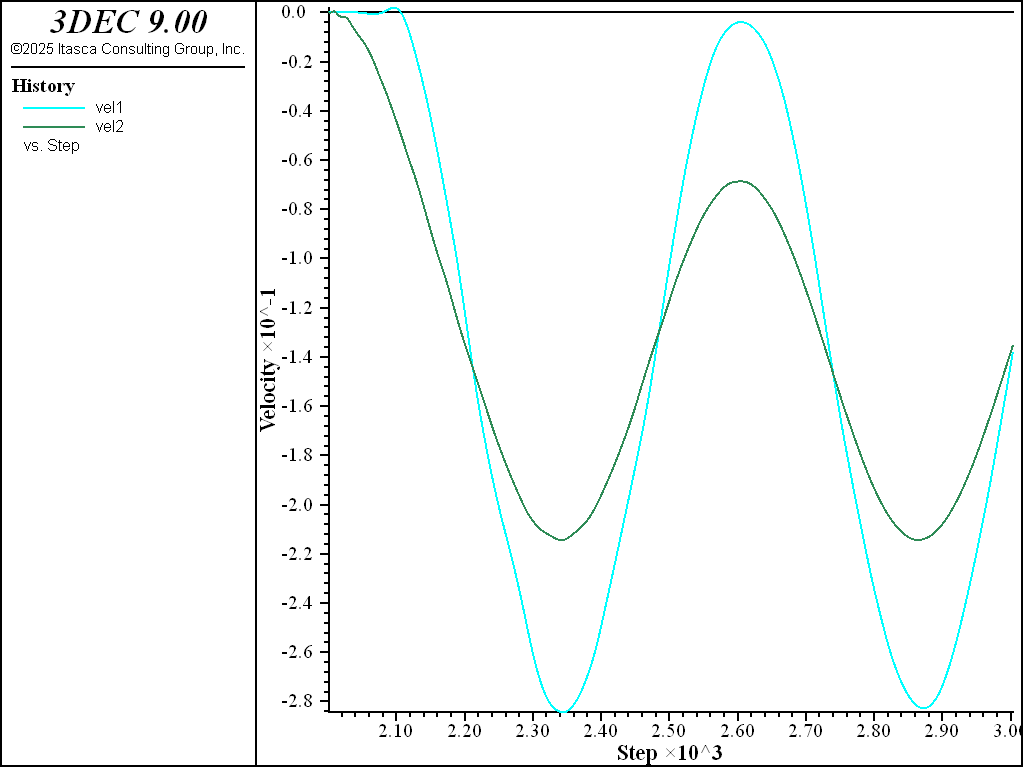
Figure 4: \(x\)-velocities of the base and dam crest using free field boundaries.
Data File - Free Field
model new
; -------------------------------------------------------------------
;
; example of dynamic free-field analysis of dam
;  impulse stress wave applied at base, free top
;
; -------------------------------------------------------------------
;
model random 10000
model configure dynamic
model large-strain on
;
model title
Dynamic Analysis of a Dam
;

; ---- geometry ----
block create brick -100 100 -100 100 -100 0

block cut joint-set dip 0 dip-direction 0 origin 0 0 -30
block hide range position-z -100 -30
block cut joint-set dip 45 dip-direction 0 origin 0 -50 0
block cut joint-set dip 45 dip-direction 180 origin 0 50 0
block hide range position-y -100 -50
block hide range position-y 50 100
block cut joint-set dip 90 dip-direction 90 origin -12 0 0
block delete range position-x -100 -12 position-z -30 0 position-y -50 50
block cut joint-set dip 51 dip-direction 90 origin -12 0 0
block delete range position-x 12 100 position-z -30 0 position-y -50 50

block group 'mat2'
block hide off
block hide range group 'mat2'
block join
block cut joint-set dip 30 dip-direction 270 ...
                    origin 30 0 -30 spacing 50 number 5
block hide off
block zone generate edgelength 26

; ---- properties ----
;
; E = 50000 MPa, v=0.25
; density = 2500 kg/m3
; cp = 4899 m/s
; cs = 2828 m/s
;
block zone cmodel assign elastic
block zone property density 0.0025  bulk 33333 shear 20000
block zone property bulk 20000 shear 12000 range group 'mat2'

block contact jmodel assign elastic
block contact property stiffness-normal 10000 stiffness-shear 4000
block contact material-table default property stiffness-normal 10000 ...
                                          stiffness-shear 4000


; --- boundary and initial conditions ---
block gridpoint apply velocity-z 0 range position-z -100
block gridpoint apply velocity-x 0 range position-x -100
block gridpoint apply velocity-x 0 range position-x 100
block gridpoint apply velocity-y 0 range position-y -100
block gridpoint apply velocity-y 0 range position-y 100
block insitu stress 0 0 0 0 0 0 gradient-z 0.00125 0.00125 0.0025 0 0 0
model gravity 0 0 -10

block mechanical damping global
model cycle 2000

block mechanical damping rayleigh 0 0 mass

history delete
model dynamic time-total 0
block gridpoint initialize displacement 0 0 0

model history mechanical unbalanced-maximum
block history name 'vel1' velocity-x position 0 0 0
block history name 'vel2' velocity-x position 0 0 -100
block history name 'vel3' velocity-x position -40 -20 -28

history name 'vel1' label 'X velocity at crest'
history name 'vel2' label 'X velocity at base'

; impulse wave to be applied to base
[freq = 15]
fish define impulse
  impulse = 0.5*(1.0-math.cos(2.0*freq*dynamic.time.total))
end
fish history impulse

model save "ff1"

model restore "ff1"

; viscous boundaries only
;
block gridpoint apply viscous-x range position-x -100
block gridpoint apply viscous-x range position-x 100
block gridpoint apply viscous-y range position-y -100
block gridpoint apply viscous-y range position-y 100

block face apply stress-xz 2.0 fish impulse range position-z -100

block gridpoint apply viscous range position-z -100
model solve time-total 0.4
model save "ff2"

model restore "ff1"

; run with Free Field Boundary
;
; --- create FF ---
;
block dynamic free-field  apply gap 10 thickness 10
block face apply stress-xz 2.0 fish impulse range position-z -100
block gridpoint apply viscous range position-z -100

history interval 1
model solve  time-total 0.4
model save "ff3"

block dynamic free-field list
| Was this helpful? ... | Itasca Software © 2024, Itasca | Updated: Nov 12, 2025 |
