Application of Dynamic Input

In 3DEC, the dynamic input can be applied in one of two ways: (a) as a prescribed velocity history; or (b) as a stress history. Option (a) enforces an exact given velocity history. If only an acceleration history is available, it must be integrated numerically to produce a velocity history for 3DEC.

The disadvantage of option (a) is that this boundary will not be an absorbing (or nonreflecting) boundary (i.e., it will reflect back into the model any outgoing stress waves). To avoid this, option (b) can be used: the velocity record is transformed into a stress record and applied to a nonreflecting (viscous) boundary. A velocity history may be converted to a stress boundary condition for similar purposes using the formula

(1)\[\sigma_n = 2\ (\rho\ C_p)\ V_n\]

or

(2)\[\sigma_s = 2 (\rho\ C_s)\ V_s\]

where:

\(\sigma_n\) = applied normal stress;

\(\sigma_s\) = applied shear stress;

\(\rho\) = mass density;

\(C_p\) = speed of p-wave propagation through medium;

\(C_s\) = speed of s-wave propagation through medium;

\(V_n\) = input normal velocity; and

\(V_s\) = input shear velocity.

Recall that \(C_p\) is given by

\[C_p = \bigl[\ (K + 4/3 G)\thinspace /\thinspace \rho\ \bigr]^{1/2}\]

and \(C_s\) is given by

\[C_s = (G\thinspace /\thinspace \rho)^{1/2}\]

The factor of two in Equations (1) and (2) accounts for the fact that the applied stress must be doubled to overcome the effect of the viscous boundary. Note that, in this case, a velocity history obtained at the boundary may be different than that from the original velocity record because of the one-dimensional approximations of Equations (1) and (2).

Baseline Correction of Input Histories

The process of “baseline correction” is performed on time histories so that the final velocity and/or displacement is zero. For example, in the figure below the velocity waveform in part (a) below might integrate to give the displacement waveform in part (b). However, it is possible to determine a low frequency wave (part (c)) which, when added to the original history, produces a final displacement that is zero (part (d)). The low frequency wave in part (c) can be a polynomial or a sine function, with free parameters that are adjusted to give the desired results.

The preceding comments really only apply to complex waveforms derived, for example, from field measurements. When using a synthetic, simple waveform, it is a simple matter to arrange the synthetic waveform itself such that the final displacement is zero. Normally, in seismic analysis, the input wave is an acceleration record. The baseline correction procedure can cause both the final velocity and displacement to be zero. (For information on standard baseline correction procedures, consult earthquake engineering texts.)

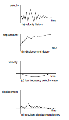
Figure 1: The baseline correction process.

An alternative to baseline correction of the input record is to apply a displacement shift at the end of the calculation if there is a residual displacement of the entire model. This can be done by applying a fixed velocity to the mesh to reduce the residual displacement to zero. This action will not affect the mechanics of the deformation of the model. Computer codes to perform baseline corrections are available from several Internet sites. For example, http://nsmp.wr.usgs.gov/processing.html provides such a code.