Analytical Thermal Formulation
Introduction
3DEC is a three-dimensional distinct element code for the analysis of problems in solid mechanics. A simple thermomechanical option has been added to the code. The main purpose of this option is to model heat sources embedded in the material. Point heat sources are placed either individually, or in lines and grids, to represent point, line or plane sources. The stress changes caused by temperature changes (due to thermal expansion) are equilibrated by using the standard mechanical 3DEC code to take a “snapshot” of the transient stresses at different times.
Note that the thermal option in 3DEC does not provide a general-purpose heat transfer program. Its purpose is specifically oriented to solving design problems associated with nuclear waste disposal.
There are several advantages to this method of calculating the temperatures:
The infinite thermal boundary is automatically incorporated.
The calculation procedure is extremely quick, compared with finite element or other numerical methods.
The calculation of the temperature at any time is independent of the temperature at previous times, so that it takes the same amount of time to calculate the solution regardless of the time at which the solution is required.
The mechanical boundary conditions can be applied correctly, because the standard mechanical logic in 3DEC is used for the mechanical part of the calculation.
Inhomogeneous and anisotropic mechanical properties can be used.
There are two limitations:
The material is assumed to be thermally homogeneous and isotropic with constant properties.
Only a few restricted thermal boundary conditions can be applied (i.e., adiabatic and isothermal planes).
In spite of the limitations of this method of solving thermal-mechanical problems, the thermal coupling in 3DEC is still a powerful aid when solving problems with heat sources, such as nuclear waste isolation problems.
Theory
The basic theoretical components of thermomechanical computations in 3DEC are the determination of the temperature distribution due to the heat sources, and the calculation of the stresses induced by these temperature changes.
The Temperature Due to a Distribution of Heat Sources
The simplest possible heat source to consider is the instantaneous point source in an infinite medium. The temperature distribution resulting from such a source is given by the simple expression (Carslaw and Jaeger 1959)
where:
\(Q\) = quantity of heat in source;
\(\rho\) = density;
\(C_p\) = specific heat;
\(K\) = thermal diffusivity = \(k/ \rho C_p\);
\(r\) = distance between source and observation point;
\(t\) = time after source released; and
\(k\) = thermal conductivity.
The temperature at a point due to any spatial and temporal distribution of heat sources can be found by considering the distribution as a sum of point sources. In the limit, as the number of sources becomes large, and the strength of each is reduced so that the total heat output is constant, the sum becomes an integral over time, space (a line, surface or volume) or both.
For example, the temperature due to a time-dependent heat source of strength \(Q(t)\) can be written as
For the case that the heat source is constant (i.e., \(Q(t)\) = \(H(t)\), where \(H(t)\) is the Heaviside step function, Equation (1) becomes (Carslaw and Jaeger 1959))
where erfc (\(x\)) = complementary error function.
The temperature due to an exponentially decaying source of the form \(Q(t) = Q_e \exp(-At)\) is given by (Crouch and McClain 1978)
where:
\(w(z) = {{2iz} \over {\pi}}\ \int_0^{\inf}\ {e^{-t^2} \over {z^2 - t^2}}\ dt,\ Im\{z\} > 0\)
\(Re\){\(z\)} = real part of \(z\)
\(Re\){\(z\)} = imaginary part of \(z\); and
\(i\) = (-1)1/2.
Line, plane and volume sources can be written as integrals of a point source over a distance, an area or a volume, respectively. In this way, completely arbitrary distributions of heat sources can be represented by analytical expressions. In 3DEC, the integration is carried out numerically, so that line sources are represented as a series of point sources along a line segment, and plane sources are represented by a grid of point sources. Thus, to determine the temperature at any point at any instant in time, a sum of terms must be computed, where each term is of the form of the right-hand side of Equation (2) or Equation (3).
Boundary Conditions
Because the point source solution used in 3DEC applies to an infinite domain, only a limited number of boundary conditions can be specified. Orthogonal isothermal planes and planes of symmetry can be specified. Symmetric planes are effected by applying an image source of equal magnitude on the opposite side of the plane of symmetry, while isothermal planes require an image source of opposite sign (a heat sink). The effect of having two equal sources is that each produces a flux across the plane, but the fluxes are in opposite directions so that the net flux is zero. Thus, symmetry planes are equivalent to adiabatic boundaries. If the sources are of opposite sign, on the other hand, the net flux is from the heat source to the heat sink. In this case, the two sources each contribute to the temperature at any point on the plane, but because the two contributions are equal in magnitude but of opposite sign, the effect is a net temperature change of zero (i.e., an isothermal condition). Figure 1 illustrates the application of adiabatic and isothermal conditions on different faces, and shows the heat source combinations required to achieve these conditions. Each boundary plane specified doubles the amount of calculation required, so that if three different planes are defined, eight times as much calculation is needed.
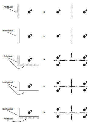
Figure 1: Adiabatic and isothermal boundaries and their 3DEC representations.
Thermally Induced Stress Changes
If a small unconstrained volume of material at a constant temperature is heated to a new temperature, it will expand, with the volume change calculated as
where:
\(\beta\) = volumetric coefficient of thermal expansion;
= \(3 \alpha\), where \(\alpha\) is the linear expansion coefficient; and
\(\Delta T\) = temperature change.
If this volume is then recompressed back to its original size, the mean stress change will be
where:
\(K\) = bulk modulus; and
\(\delta_{ij}\) = Kronecker delta function (1 for \(i\) = \(j\); 0, otherwise).
The negative sign reflects the convention that compressive stresses are negative.
The thermally induced stresses need not be in equilibrium since they depend solely on temperature changes. If they are not in equilibrium, the medium will move to restore equilibrium. For example, if two thin metal plates are bolted together but separated by a thin insulator and one is heated, the thermally induced stresses in the heated plate will cause it to expand, producing bending as the other plate resists the motion. One plate will be in tension, and the other in compression.
Application in 3DEC
Heat source characteristics such as number of components, decay constants and proportion of each component are input by the user. In addition, the location and initial strengths of arrays of point sources are input. Symmetric and isothermal planes may be specified, as may the initial temperature and the time at which the solution is desired. Once all these quantities have been input, the temperatures are calculated at all gridpoints. Stresses are not calculated at this stage, but when mechanical cycling is performed, the average temperature change for each zone is used to calculate a stress change in each zone. The stress state thus produced will not be in equilibrium, but is treated as an initial condition for the mechanical calculation. The standard 3DEC mechanical calculation is used to reach equilibrium.
Input Commands
The commands required for solving thermal-mechanical problems with 3DEC are given below. The commands are presented in groups corresponding to their function. It is assumed that the reader is familiar with |3dec| and the mechanical calculations it performs, as well as the input commands.
|
Verification
First, the temperature distribution due to a single point source is compared with an analytical solution. Then, to test the thermal logic thoroughly, different combinations of point, line and grid sources are examined. These results should be expected to agree extremely well with the analytical solutions, since 3DEC is essentially just evaluating the analytical solutions. These first examples merely confirm that the coding is correct, and illustrate the use of the program.
Finally, the correctness of the mechanical solution is demonstrated by comparing the stress state due to a point source with that of a point source in an infinite medium. This is a true test of the thermomechanical coupling, since the 3DEC mechanical logic is used to equilibrate the stresses. This test is particularly rigorous because the analytical solution contains a singularity at the source itself, producing steep gradients around the source.
A Single Non-decaying Point Heat Source
Consider a 30 kW heat source, located at the origin, in an infinite medium with the following properties:
density |
1500 kg/m3 |
specific heat |
500 J/kg/C0 |
thermal conductivity |
2.4 W/m/C0 |
From these properties, a thermal diffusivity of 3.2 × 10⁻⁶ m2/s is calculated.
The following data file is used to calculate the temperature distribution due to this source. The accuracy of thermal calculations in 3DEC is independent of the mechanical grid, but the temperatures are calculated at gridpoints, so a grid from which the calculated temperature distribution can be extracted is specified.
PointSource.dat
model new
model configure thermal
block thermal analytical on
block create brick 0,2 0,2 0,10
block cut joint-set dip 0 dip-direction 0 origin 0 0 2 spacing 2
block zone generate edgelength 3.5
block thermal source 1, number-components 2, component 1 = fraction .2, ...
  component 2 = fraction .8
block thermal analytical diffusivity=3.2e-6 conductivity=2.4
block thermal analytical tolerance 0.01
block thermal point 0,0,0 source 1 strength 30000 time-start 0

fish define get_temp(itab)
;
; Put temperatures into input table
;
  loop foreach local gp block.gp.list
    local radius = math.mag(block.gp.pos(gp))
    if radius >= 2.0
      table(itab,radius) = block.gp.temp(gp)
    end_if
  end_loop
end

program call "solutions.fis"
block thermal analytical solve time=2e6
[get_temp(1)] ; table '1' is 3DEC results at 2e6 s
table '1' label '2e6 s - 3DEC'
[point_source_line(2e6,2,30000)] ; table '2' is analytical results at 2e6 s
table '2' label '2e6 s - Analytical'

block thermal analytical solve time=2e7
[get_temp(3)] ; table '3' is 3DEC results at 2e7 s
table '3' label '2e7 s - 3DEC'
[point_source_line(2e7,4,30000)] ; table '4' is analytical results at 2e7 s
table '4' label '2e7 s - Analytical'

block thermal analytical solve time=2e11
[get_temp(5)] ; table '5' is 3DEC results at 2e11 s
table '5' label '2e11 s - 3DEC'
[point_source_line(2e11,6,30000)] ; table '6' is analytical results at 2e11 s
table '6' label '2e11 s - Analytical'
Figure 2 shows the results of the 3DEC calculations compared with the analytical solution, which is obtained using Equation (2). 3DEC uses an analytical expression for the temperature calculations, so it would be expected that the temperatures would agree exactly. The slight differences are due to the methods of calculating the complementary error function, erfc(\(x\)). This function is not readily available in computer languages, but must be approximated by polynomials. The polynomial used to evaluate the analytical solution differs from that used in 3DEC. The difference is less than one percent everywhere, except at the last few points for a time of 2e6 seconds, where the temperatures are so small that the difference is not significant. Note that temperatures are only shown at a distance of 2 m from the source because, if placed closer than this, the singularity at the source location would dominate the figure.
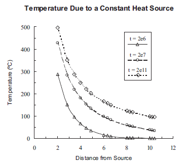
Figure 2: Temperature distribution around a constant heat source.
Superposition of Several Non-decaying Sources
This data file illustrates the superposition of four different sources, with different strengths and starting times. Once again, the solution is compared with the analytic solution (Table 3), and, again, the 3DEC results are in excellent agreement. The largest errors are located where only small temperature changes occur.
SeveralSources.dat
model new
model configure thermal
block thermal analytical on
block create brick 0,2 0,2 0,20
block cut joint-set dip 0 dip-direction 0 origin 0 0 2 spacing 2
block zone generate edgelength 3.5

; use two different source specifications to test summing
block thermal source 1, number-components 2, component 1 = fraction .2 ...
  component 2 = fraction .8
block thermal source 2, number-components 2, component 1 = fraction .4 ...
  component 2 = fraction .6
block thermal analytical diffusivity=3.2e-6 conductivity=2.4
block thermal analytical tolerance 0.01

fish define sources
  global pos1 = vector(2,2,10)
  global pos2 = vector(1,2,10)
  global pos3 = vector(2,1,10)
  global pos4 = vector(2,2,5)
  global str1 = 7000
  global str2 = 10000
  global str3 = 4000
  global str4 = 9000
  global ttime1 = 1e7
  global ttime2 = 1e7
  global ttime3 = 2e7
  global ttime4 = 3e7
end
[sources]

block thermal point 2,2,10 source 1 strength [str1] time-start [ttime1]
block thermal point 1,2,10 source 2 strength [str2] time-start [ttime2]
block thermal point 2,1,10 source 1 strength [str3] time-start [ttime3]
block thermal point 2,2,5 source 2 strength [str4] time-start [ttime4]

fish define get_temp(itab)
;
; Put temperatures into input table
;
  loop foreach local gp block.gp.list
    local radius = math.mag(block.gp.pos(gp))
    if radius >= 2.0
      table(itab,radius) = block.gp.temp(gp)
    end_if
  end_loop
end

; t less than 0 forigin all sources
block thermal analytical solve time=8e6

; t = 2e6 forigin 2 sources
block thermal analytical solve time=1.2e7
program call "solutions.fis"
program call "four_sources.fis"
[four_sources(1.2e7)]

; t=2e7 forigin two, 1e7 forigin 1, 0 forigin the other
block thermal analytical solve time=3e7
[four_sources(3e7)]
X Y Z |
\(t\) = 1.2\(e\)7 |
\(t\) = 3\(e\)7 |
||||
|---|---|---|---|---|---|---|
3DEC |
Analytical |
% error |
3DEC |
Analytical |
% error |
|
0 2 0 |
0.26 |
0.29 |
-8.8 |
23.31 |
23.32 |
-0.04 |
2 2 0 |
0.28 |
0.31 |
-8.2 |
23.86 |
23.87 |
-0.04 |
2 0 0 |
0.23 |
0.26 |
-9.8 |
22.93 |
22.95 |
-0.08 |
0 0 0 |
0.22 |
0.24 |
-10.5 |
22.41 |
22.42 |
-0.06 |
0 0 2 |
1.29 |
1.30 |
-0.4 |
35.65 |
35.64 |
0.02 |
2 0 2 |
1.40 |
1.41 |
-0.2 |
36.75 |
36.74 |
0.01 |
0 2 2 |
1.59 |
1.59 |
0.04 |
37.47 |
37.47 |
0.01 |
2 2 2 |
1.73 |
1.73 |
0.2 |
38.65 |
38.64 |
0.03 |
2 2 4 |
8.48 |
8.44 |
0.4 |
65.00 |
64.95 |
0.08 |
0 2 4 |
7.69 |
7.65 |
0.5 |
62.12 |
62.07 |
0.07 |
2 0 4 |
6.64 |
6.60 |
0.6 |
60.48 |
60.43 |
0.08 |
0 0 4 |
6.04 |
6.00 |
0.6 |
57.87 |
57.83 |
0.07 |
2 2 4 |
8.48 |
8.44 |
0.4 |
65.00 |
64.95 |
0.08 |
0 2 4 |
7.69 |
7.65 |
0.5 |
62.12 |
62.07 |
0.08 |
2 0 4 |
6.64 |
6.60 |
0.6 |
60.48 |
60.43 |
0.08 |
0 0 4 |
6.04 |
6.00 |
0.6 |
57.87 |
57.83 |
0.07 |
0 0 6 |
22.59 |
22.6 |
-0.1 |
97.5 |
97.43 |
0.07 |
2 0 6 |
25.45 |
25.5 |
-0.2 |
105.0 |
105.0 |
0.03 |
0 2 6 |
31.0 |
31.1 |
-0.2 |
109.9 |
109.8 |
0.07 |
2 2 6 |
35.33 |
35.4 |
-0.2 |
119.0 |
119.0 |
0.03 |
0 0 6 |
22.59 |
22.6 |
-0.1 |
97.5 |
97.4 |
0.07 |
2 0 6 |
25.45 |
25.5 |
-0.2 |
105.0 |
105.0 |
0.03 |
0 2 6 |
31.0 |
31.1 |
-0.2 |
109.9 |
109.8 |
0.07 |
2 2 6 |
35.33 |
35.4 |
-0.2 |
119.0 |
119.0 |
0.03 |
2 2 8 |
145.7 |
145.7 |
0.03 |
271.1 |
271.1 |
-0.01 |
0 2 8 |
114.1 |
114.1 |
0.02 |
222.2 |
222.2 |
-0.007 |
2 0 8 |
79.62 |
79.7 |
-0.05 |
199.5 |
199.5 |
-0.007 |
0 0 8 |
66.71 |
66.8 |
-0.09 |
169.6 |
169.5 |
0.03 |
2 2 8 |
145.7 |
145.7 |
0.03 |
271.1 |
271.1 |
-0.01 |
0 2 8 |
114.1 |
114.1 |
0.02 |
222.2 |
222.2 |
-0.007 |
2 0 8 |
79.62 |
79.7 |
-0.05 |
199.5 |
199.5 |
-0.007 |
0 0 8 |
66.71 |
66.8 |
-0.09 |
169.6 |
169.5 |
0.03 |
2 2 10 |
23420 |
23410 |
0.01 |
23620 |
23621 |
-0.007 |
0 2 10 |
325.4 |
325.4 |
-0.002 |
454.2 |
454.4 |
-0.05 |
2 0 10 |
145.7 |
145.7 |
0.03 |
344.3 |
344.4 |
-0.02 |
0 0 10 |
114.1 |
114.1 |
0.02 |
237.2 |
237.2 |
0.002 |
Lines and Grids of Sources
To verify the operation of the commands to generate lines and grids of sources, one problem is solved with three different sets of data. The first file uses points only, the second uses lines, and the third uses grids. Note how the use of the grid and line commands drastically reduces the amount of input required. It can easily be verified that these three data sets generate the same temperature distribution.
Data Files
AnalyticalGrid/points.dat
;
; collection of thermal point sources
;
model new
model configure thermal
block thermal analytical on
block create brick 0,2 0,10 0,2
block cut joint-set dip 90 dip-direction 0 origin 0 2 0 spacing 2
block zone generate edgelength 3.5

; Use three different source specifications
block thermal source 1 number-components 2, component 1 fraction .2 ...
  component 2 fraction .8
block thermal source 2 number-components 3, component 1 fraction .3 ...
  component 2 fraction .5, component 3 fraction .2
block thermal source 3 number-components 1, component 1 fraction 1

block thermal analytical diffusivity=3.2e-6 conductivity=2.4
block thermal analytical tolerance 0.01

;
block thermal point 0.5 0.5 0.5 source 1 strength 3000   time-start 1e7
block thermal point 0.5 0.5 0.5 source 2 strength 4000   time-start 2e7
block thermal point 0.5 0.5 0.5 source 3 strength 5000   time-start 0
;
block thermal point 0.5 1.0 0.5 source 1 strength 3000   time-start 1e7
block thermal point 0.5 1.0 0.5 source 2 strength 4000   time-start 2e7
block thermal point 0.5 1.0 0.5 source 3 strength 5000   time-start 0
;
block thermal point 0.5 1.5 0.5 source 1 strength 3000   time-start 1e7
block thermal point 0.5 1.5 0.5 source 2 strength 4000   time-start 2e7
block thermal point 0.5 1.5 0.5 source 3 strength 5000   time-start 0
;
block thermal point 0.5 0.5 1.0 source 1 strength 3000   time-start 1e7
block thermal point 0.5 0.5 1.0 source 2 strength 4000   time-start 2e7
block thermal point 0.5 0.5 1.0 source 3 strength 5000   time-start 0
;
block thermal point 0.5 1.0 1.0 source 1 strength 3000   time-start 1e7
block thermal point 0.5 1.0 1.0 source 2 strength 4000   time-start 2e7
block thermal point 0.5 1.0 1.0 source 3 strength 5000   time-start 0
;
block thermal point 0.5 1.5 1.0 source 1 strength 3000   time-start 1e7
block thermal point 0.5 1.5 1.0 source 2 strength 4000   time-start 2e7
block thermal point 0.5 1.5 1.0 source 3 strength 5000   time-start 0
;
block thermal point 0.5 0.5 1.5 source 1 strength 3000   time-start 1e7
block thermal point 0.5 0.5 1.5 source 2 strength 4000   time-start 2e7
block thermal point 0.5 0.5 1.5 source 3 strength 5000   time-start 0
;
block thermal point 0.5 1.0 1.5 source 1 strength 3000   time-start 1e7
block thermal point 0.5 1.0 1.5 source 2 strength 4000   time-start 2e7
block thermal point 0.5 1.0 1.5 source 3 strength 5000   time-start 0
;
block thermal point 0.5 1.5 1.5 source 1 strength 3000   time-start 1e7
block thermal point 0.5 1.5 1.5 source 2 strength 4000   time-start 2e7
block thermal point 0.5 1.5 1.5 source 3 strength 5000   time-start 0
;
block thermal point 1.0 0.5 0.5 source 1 strength 3000   time-start 1e7
block thermal point 1.0 0.5 0.5 source 2 strength 4000   time-start 2e7
block thermal point 1.0 0.5 0.5 source 3 strength 5000   time-start 0
;
block thermal point 1.0 1.0 0.5 source 1 strength 3000   time-start 1e7
block thermal point 1.0 1.0 0.5 source 2 strength 4000   time-start 2e7
block thermal point 1.0 1.0 0.5 source 3 strength 5000   time-start 0
;
block thermal point 1.0 1.5 0.5 source 1 strength 3000   time-start 1e7
block thermal point 1.0 1.5 0.5 source 2 strength 4000   time-start 2e7
block thermal point 1.0 1.5 0.5 source 3 strength 5000   time-start 0
;
block thermal point 1.0 0.5 1.0 source 1 strength 3000   time-start 1e7
block thermal point 1.0 0.5 1.0 source 2 strength 4000   time-start 2e7
block thermal point 1.0 0.5 1.0 source 3 strength 5000   time-start 0
;
block thermal point 1.0 1.0 1.0 source 1 strength 3000   time-start 1e7
block thermal point 1.0 1.0 1.0 source 2 strength 4000   time-start 2e7
block thermal point 1.0 1.0 1.0 source 3 strength 5000   time-start 0
;
block thermal point 1.0 1.5 1.0 source 1 strength 3000   time-start 1e7
block thermal point 1.0 1.5 1.0 source 2 strength 4000   time-start 2e7
block thermal point 1.0 1.5 1.0 source 3 strength 5000   time-start 0
;
block thermal point 1.0 0.5 1.5 source 1 strength 3000   time-start 1e7
block thermal point 1.0 0.5 1.5 source 2 strength 4000   time-start 2e7
block thermal point 1.0 0.5 1.5 source 3 strength 5000   time-start 0
;
block thermal point 1.0 1.0 1.5 source 1 strength 3000   time-start 1e7
block thermal point 1.0 1.0 1.5 source 2 strength 4000   time-start 2e7
block thermal point 1.0 1.0 1.5 source 3 strength 5000   time-start 0
;
block thermal point 1.0 1.5 1.5 source 1 strength 3000   time-start 1e7
block thermal point 1.0 1.5 1.5 source 2 strength 4000   time-start 2e7
block thermal point 1.0 1.5 1.5 source 3 strength 5000   time-start 0
;
block thermal point 1.5 0.5 0.5 source 1 strength 3000   time-start 1e7
block thermal point 1.5 0.5 0.5 source 2 strength 4000   time-start 2e7
block thermal point 1.5 0.5 0.5 source 3 strength 5000   time-start 0
;
block thermal point 1.5 1.0 0.5 source 1 strength 3000   time-start 1e7
block thermal point 1.5 1.0 0.5 source 2 strength 4000   time-start 2e7
block thermal point 1.5 1.0 0.5 source 3 strength 5000   time-start 0
;
block thermal point 1.5 1.5 0.5 source 1 strength 3000   time-start 1e7
block thermal point 1.5 1.5 0.5 source 2 strength 4000   time-start 2e7
block thermal point 1.5 1.5 0.5 source 3 strength 5000   time-start 0
;
block thermal point 1.5 0.5 1.0 source 1 strength 3000   time-start 1e7
block thermal point 1.5 0.5 1.0 source 2 strength 4000   time-start 2e7
block thermal point 1.5 0.5 1.0 source 3 strength 5000   time-start 0
;
block thermal point 1.5 1.0 1.0 source 1 strength 3000   time-start 1e7
block thermal point 1.5 1.0 1.0 source 2 strength 4000   time-start 2e7
block thermal point 1.5 1.0 1.0 source 3 strength 5000   time-start 0
;
block thermal point 1.5 1.5 1.0 source 1 strength 3000   time-start 1e7
block thermal point 1.5 1.5 1.0 source 2 strength 4000   time-start 2e7
block thermal point 1.5 1.5 1.0 source 3 strength 5000   time-start 0
;
block thermal point 1.5 0.5 1.5 source 1 strength 3000   time-start 1e7
block thermal point 1.5 0.5 1.5 source 2 strength 4000   time-start 2e7
block thermal point 1.5 0.5 1.5 source 3 strength 5000   time-start 0
;
block thermal point 1.5 1.0 1.5 source 1 strength 3000   time-start 1e7
block thermal point 1.5 1.0 1.5 source 2 strength 4000   time-start 2e7
block thermal point 1.5 1.0 1.5 source 3 strength 5000   time-start 0
;
block thermal point 1.5 1.5 1.5 source 1 strength 3000   time-start 1e7
block thermal point 1.5 1.5 1.5 source 2 strength 4000   time-start 2e7
block thermal point 1.5 1.5 1.5 source 3 strength 5000   time-start 0

block thermal analytical solve time=2.2e7
program log-file "points-temp.log"
program log on
block gridpoint list temperature
program log off
AnalyticalGrid/points.dat
;
; collection of thermal line sources
;
model new
model configure thermal
block thermal analytical on
block create brick 0,2 0,10 0,2
block cut joint-set dip 90 dip-direction 0 origin 0 2 0 spacing 2
block zone generate edgelength 3.5

; Use three different source specifications
block thermal source 1 number-components 2, component 1 fraction .2 ...
  component 2 fraction .8
block thermal source 2 number-components 3, component 1 fraction .3 ...
  component 2 fraction .5, component 3 fraction .2
block thermal source 3 number-components 1, component 1 fraction 1

block thermal analytical diffusivity=3.2e-6 conductivity=2.4
block thermal analytical tolerance 0.01

;
block thermal line point-1 0.5 0.5 0.5 point-2 1.5 0.5 0.5 ...
                   source 1 strength 3000   time-start 1e7 n12=3
block thermal line point-1 0.5 0.5 0.5 point-2 1.5 0.5 0.5 ...
                   source 2 strength 4000   time-start 2e7 n12=3
block thermal line point-1 0.5 0.5 0.5 point-2 1.5 0.5 0.5 ...
                   source 3 strength 5000   time-start 0   n12=3
;
block thermal line point-1 0.5 0.5 1.0 point-2 1.5 0.5 1.0 ...
                   source 1 strength 3000   time-start 1e7 n12=3
block thermal line point-1 0.5 0.5 1.0 point-2 1.5 0.5 1.0 ...
                   source 2 strength 4000   time-start 2e7 n12=3
block thermal line point-1 0.5 0.5 1.0 point-2 1.5 0.5 1.0 ...
                   source 3 strength 5000   time-start 0   n12=3
;
block thermal line point-1 0.5 0.5 1.5 point-2 1.5 0.5 1.5 ...
                   source 1 strength 3000   time-start 1e7 n12=3
block thermal line point-1 0.5 0.5 1.5 point-2 1.5 0.5 1.5 ...
                   source 2 strength 4000   time-start 2e7 n12=3
block thermal line point-1 0.5 0.5 1.5 point-2 1.5 0.5 1.5 ...
                   source 3 strength 5000   time-start 0   n12=3
;
;
block thermal line point-1 0.5 1.0 0.5 point-2 0.5 1.0 1.5 ...
                   source 1 strength 3000   time-start 1e7 n12=3
block thermal line point-1 0.5 1.0 0.5 point-2 0.5 1.0 1.5 ...
                   source 2 strength 4000   time-start 2e7 n12=3
block thermal line point-1 0.5 1.0 0.5 point-2 0.5 1.0 1.5 ...
                   source 3 strength 5000   time-start 0   n12=3
;
block thermal line point-1 1.0 1.0 0.5 point-2 1.0 1.0 1.5 ...
                   source 1 strength 3000   time-start 1e7 n12=3
block thermal line point-1 1.0 1.0 0.5 point-2 1.0 1.0 1.5 ...
                   source 2 strength 4000   time-start 2e7 n12=3
block thermal line point-1 1.0 1.0 0.5 point-2 1.0 1.0 1.5 ...
                   source 3 strength 5000   time-start 0   n12=3
;
block thermal line point-1 1.5 1.0 0.5 point-2 1.5 1.0 1.5 ...
                   source 1 strength 3000   time-start 1e7 n12=3
block thermal line point-1 1.5 1.0 0.5 point-2 1.5 1.0 1.5 ...
                   source 2 strength 4000   time-start 2e7 n12=3
block thermal line point-1 1.5 1.0 0.5 point-2 1.5 1.0 1.5 ...
                   source 3 strength 5000   time-start 0   n12=3
;
block thermal line point-1 0.5 1.5 0.5 point-2 0.5 1.5 1.5 ...
                   source 1 strength 3000   time-start 1e7 n12=3
block thermal line point-1 0.5 1.5 0.5 point-2 0.5 1.5 1.5 ...
                   source 2 strength 4000   time-start 2e7 n12=3
block thermal line point-1 0.5 1.5 0.5 point-2 0.5 1.5 1.5 ...
                   source 3 strength 5000   time-start 0   n12=3
;
block thermal line point-1 1.0 1.5 0.5 point-2 1.0 1.5 1.5 ...
                   source 1 strength 3000   time-start 1e7 n12=3
block thermal line point-1 1.0 1.5 0.5 point-2 1.0 1.5 1.5 ...
                   source 2 strength 4000   time-start 2e7 n12=3
block thermal line point-1 1.0 1.5 0.5 point-2 1.0 1.5 1.5 ...
                   source 3 strength 5000   time-start 0   n12=3
;
block thermal line point-1 1.5 1.5 0.5 point-2 1.5 1.5 1.5 ...
                   source 1 strength 3000 time-start 1e7 n12=3
block thermal line point-1 1.5 1.5 0.5 point-2 1.5 1.5 1.5 ...
                   source 2 strength 4000 time-start 2e7 n12=3
block thermal line point-1 1.5 1.5 0.5 point-2 1.5 1.5 1.5 ...
                   source 3 strength 5000 time-start 0   n12=3

block thermal analytical solve time=2.2e7
program log-file "lines-temp.log"
program log on
block gridpoint list temperature
program log off
AnalyticalGrid/grids.dat
;
; collection of thermal line sources
;
model new
model configure thermal
block thermal analytical on
block create brick 0,2 0,10 0,2
block cut joint-set dip 90 dip-direction 0 origin 0 2 0 spacing 2
block zone generate edgelength 3.5

; Use three different source specifications
block thermal source 1 number-components 2, component 1 fraction .2 ...
  component 2 fraction .8
block thermal source 2 number-components 3, component 1 fraction .3 ...
  component 2 fraction .5, component 3 fraction .2
block thermal source 3 number-components 1, component 1 fraction 1

block thermal analytical diffusivity=3.2e-6 conductivity=2.4
block thermal analytical tolerance 0.01

;
block thermal grid point-1 (0.5 0.5 0.5) point-2 (0.5 0.5 1.5) ...
                   point-3 (1.5 0.5 1.5) n12=3 n23=3 source 1 ...
                   strength 3000 time-start 1e7
block thermal grid point-1 (0.5 0.5 0.5) point-2 (0.5 0.5 1.5) ...
                   point-3 (1.5 0.5 1.5) n12=3 n23=3 source 2 ...
                   strength 4000 time-start 2e7
block thermal grid point-1 (0.5 0.5 0.5) point-2 (0.5 0.5 1.5) ...
                   point-3 (1.5 0.5 1.5) n12=3 n23=3 source 3 ...
                   strength 5000 time-start 0
;
block thermal grid point-1 (0.5 1.0 0.5) point-2 (0.5 1.0 1.5) ...
                   point-3 (0.5 1.5 1.5) n12=3 n23=2 source 1 ...
                   strength 3000 time-start 1e7
block thermal grid point-1 (0.5 1.0 0.5) point-2 (0.5 1.0 1.5) ...
                   point-3 (0.5 1.5 1.5) n12=3 n23=2 source 2 ...
                   strength 4000 time-start 2e7
block thermal grid point-1 (0.5 1.0 0.5) point-2 (0.5 1.0 1.5) ...
                   point-3 (0.5 1.5 1.5) n12=3 n23=2 source 3 ...
                   strength 5000 time-start 0
;
block thermal grid point-1 (1.0 1.0 0.5) point-2 (1.0 1.0 1.5) ...
                   point-3 (1.0 1.5 1.5) n12=3 n23=2 source 1 ...
                   strength 3000 time-start 1e7
block thermal grid point-1 (1.0 1.0 0.5) point-2 (1.0 1.0 1.5) ...
                   point-3 (1.0 1.5 1.5) n12=3 n23=2 source 2 ...
                   strength 4000 time-start 2e7
block thermal grid point-1 (1.0 1.0 0.5 point-2 )(1.0 1.0 1.5) ...
                   point-3 (1.0 1.5 1.5) n12=3 n23=2 source 3 ...
                   strength 5000 time-start 0
;
block thermal grid point-1 (1.5 1.0 0.5) point-2 (1.5 1.0 1.5) ...
                   point-3 (1.5 1.5 1.5) n12=3 n23=2 source 1 ...
                   strength 3000 time-start 1e7
block thermal grid point-1 (1.5 1.0 0.5) point-2 (1.5 1.0 1.5) ...
                   point-3 (1.5 1.5 1.5) n12=3 n23=2 source 2 ...
                   strength 4000 time-start 2e7
block thermal grid point-1 (1.5 1.0 0.5) point-2 (1.5 1.0 1.5) ...
                   point-3 (1.5 1.5 1.5) n12=3 n23=2 source 3 ...
                   strength 5000 time-start 0

block thermal analytical solve time=2.2e7
program log-file "grids-temp.log"
program log on
block gridpoint list temperature
program log off
Decaying Sources
The following data file demonstrates the solution for a decaying heat source.
AnalyticalDecayingdecaying-source.dat
;
; thermal simulation of a decaying point sources
;
model new
model configure thermal
block thermal analytical on
block create brick 0,2 0,10 0,2
block cut joint-set dip 90 dip-direction 0 origin 0 2 0 spacing 2
block zone generate edgelength 3.5

block thermal source 1 number-components 2 ...
  component 1 fraction .2 decay 1.5 ...
  component 2 fraction .8 decay 1.5

block thermal analytical diffusivity=.166667 conductivity 5
block thermal analytical tolerance 0.01

block thermal point 0 0 0 source 1 strength 62.8318e3 time-start 0

block thermal analytical solve time=6

fish define get_temp(itab)
;
; Put temperatures into input table
;
  loop foreach local gp block.gp.list
    local radius = math.mag(block.gp.pos(gp))
    if radius >= 2.0
      table(itab,radius) = block.gp.temp(gp)
    end_if
  end_loop
end


[get_temp(1)] ; table '1' is 3DEC results at 6 s
The resulting temperature distribution is shown in Figure 3. The solution was checked against that given by Equation (3), using tabulated values of \(w(z)\) found in Abramowitz and Stegun (1972). 3DEC agrees extremely well with the analytical solution.
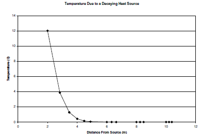
Figure 3: Temperature distribution around a decaying heat source.
Thermomechanical Effects
The primary purpose of the thermal logic in 3DEC is to examine thermomechanical effects, not just thermal effects. To test this capability, the response of an infinite medium to an instantaneous point source is determined.
Nowacki (1962) gives the solution for an instantaneous point source in an infinite medium as
where:
\(\phi(R,t) = {mQ \over {4 \pi R}} \ \hbox{erf} \ \bigl[{K \over {(\beta^{1/2}}} \bigr]\);
\(R\) = distance from source;
\(t\) = time;
\(m\) = \({\alpha (1 + \nu)} \over {(1 - \nu)}\) ;
\(\nu\) = Poisson’s ratio;
\(G\) = shear modulus;
\(\beta\) = 4 \(Kt\);
\(K\) = thermal diffusivity;
\(Q\) = “source strength”; = \(Q_o / \rho\ C_p\);
\(Qo\) = heat released (\(J\));
\(\rho\) = density;
\(Cp\) = specific heat; and
\(\alpha\) = thermal-expansion coefficient.
From these equations, we can obtain the stresses and displacements along the \(z\)-axis (\(x = y\) = 0):
where:
\(V_1(z,t) = Q\ \hbox{erf} \ \bigl[{z \over {(\beta)^{1/2}}} \bigr]\);
\(V_2(z,t) = \bigl[{Q \over {(\beta)^{1/2}}} \ \hbox{exp}(-z^2/\beta) \bigr]\); and
\(V_3(z,t) = V_2(z,t)/\beta\)
The following material properties and source parameters are used to solve this problem with 3DEC:
thermal conductivity |
1 W/m/°C |
density |
2000 kg/m3 |
specific heat |
500 J/kg/°C |
linear thermal-expansion coefficient |
5 × 10⁻³ /°C |
Young’s modulus |
1.01 GPa |
Poisson’s ratio |
0.2 |
The total heat input is 108 J , which in 3DEC is represented by a 100 kW source acting for 1000 seconds. A cube of side 5 m is used to represent one octant of the medium, as shown in Figure 4. For the times at which the solution is obtained here (1 day and 3 days), the model is large enough to reduce the effect of the boundaries.
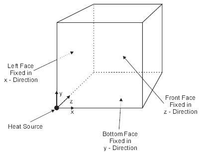
Figure 4: Conceptual representation of 3DEC block for modeling effect of point heat source.
The data file for this problem is shown:
AnalyticalCoupled/thermomechanical.dat
model new
fish automatic-create off
model large-strain on
;
; Data file forigin thermomechanical verification of 3DEC
;
model configure thermal
block thermal analytical on
;
; define 5 m by 5 m by 5 m region to represent one octant of
; infinite domain
block create brick 0 5 0 5 0 5
;
; define joints so that grid can be refined nearer to source
block cut joint-set origin .5 .5 .5 dip 0 dip-direction 0
block cut joint-set origin .5 .5 .5 dip 90 dip-direction 0
block cut joint-set origin .5 .5 .5 dip 90 dip-direction 90
block cut joint-set origin 1.5 1.5 1.5 dip 0 dip-direction 0
block cut joint-set origin 1.5 1.5 1.5 dip 90 dip-direction 0
block cut joint-set origin 1.5 1.5 1.5 dip 90 dip-direction 90
block cut joint-set origin 2.5 2.5 2.5 dip 0 dip-direction 0
block cut joint-set origin 2.5 2.5 2.5 dip 90 dip-direction 0
block cut joint-set origin 2.5 2.5 2.5 dip 90 dip-direction 90

; join all blocks to create a continuum and generate zoning
block join
block zone generate edgelength 0.125 ...
  range position-x 0,0.5 position-y 0,0.5 position-z 0,0.5
block zone generate edgelength 0.25 ...
  range position-x 0,1.5 position-y 0,1.5 position-z 0,1.5
block zone generate edgelength 0.5 ...
  range position-x 0,2.5 position-y 0,2.5 position-z 0,2.5
block zone generate edgelength 1.0 ...
  range position-x 0,5.0 position-y 0,5.0 position-z 0,5.0
model save "gen"

model restore "gen"

fish define parameters
  global bulk_ = 5.6e8
  global shear_ = 4.2e8
  global dens_ = 2000.0
  global alpha = 5e-3 ; thermal expansion coefficient
  global Cp = 500.0 ; specific heat
  global cond_ = 1.0 ; conductivity
  global Q0 = 1e8 ; 100 kW * 1000 seconds

  global diff_ = cond_ / (dens_*Cp) ; diffusivity
end
[parameters]

; Define material properties
block zone cmodel assign elastic
block zone property density [dens_] bulk=[bulk_] shear=[shear_]
block zone thermal property expansion [alpha]

block contact material-table default property stiffness-normal 10 ...
                                          stiffness-shear 10

block thermal analytical conductivity [cond_] diffusivity [diff_]

; mechanical symmetry
block gridpoint apply velocity-x 0 range position-x 0
block gridpoint apply velocity-y 0 range position-y 0
block gridpoint apply velocity-z 0 range position-z 0

; fixed far boundary (only used forigin seconductivitycase)
block gridpoint apply velocity-x 0 range position-x 5
block gridpoint apply velocity-y 0 range position-y 5
block gridpoint apply velocity-z 0 range position-z 5

; define heat source in bottom left corner of octant
; (100 kW forigin 1000 seconds)
block thermal source 1 number-components 1 component 1 fraction 1
block thermal point 0 0 0 source 1 strength 1e5 time-start 0
block thermal point 0 0 0 source 1 strength -1e5 time-start 1000

; results after 1 day
block thermal analytical solve time=8.64e4
model solve

fish define get_3dec(itab_sxx, itab_syy, itab_szz, itab_dis)
;
; Put stresses and displacements into tables
;
  block.field.method.name = 'average'
  loop local i (1,20)
    local dist = i*0.25
    block.field.name = 'stress-xx'
    table(itab_sxx,dist) = block.field.get(0.0,0.0,dist)
    block.field.name = 'stress-yy'
    table(itab_syy,dist) = block.field.get(0.0,0.0,dist)
    block.field.name = 'stress-zz'
    table(itab_szz,dist) = block.field.get(0.0,0.0,dist)
    block.field.name = 'displacement-z'
    table(itab_dis,dist) = block.field.get(0.0,0.0,dist)
  end_loop
end
[get_3dec(1,3,5,7)]

; fill even numbered tables with analytical solution
program call "thermomechanical-solution.fis"
[analytical(2,4,6,8,8.64e4)]

table '1' label 'SXX 3DEC'
table '2' label 'SXX Analytical'
table '3' label 'SYY 3DEC'
table '4' label 'SYY Analytical'
table '5' label 'SZZ 3DEC'
table '6' label 'SZZ Analytical'
table '7' label 'Disp 3DEC'
table '8' label 'Disp Analytical'

model save "tmtest-1day"

table '1' clear
table '2' clear
table '3' clear
table '4' clear
table '5' clear
table '6' clear
table '7' clear
table '8' clear

; results after 3 days
block thermal analytical solve time=2.592e5
model solve

[get_3dec(1,3,5,7)]
[analytical(2,4,6,8,2.592e5)]

model save "tmtest-3days"
The block plot from 3DEC is shown in Figure 5. The discretization is finer near the source, where stress and displacement gradients are greatest.
Figure 6 shows the comparison between \(\sigma_{zz}\) calculated by 3DEC, and the analytical solution near the \(z\)-axis (\(x = y\) = 0). Figure 7 and Figure 8 show similar plots for \(\sigma_{xx}\) and \(\sigma_{yy}\), while Figure 9 shows the displacements. On each of these plots, two different cases are shown: one where the outer boundaries are free to move; and another where the outer boundaries are fixed against movement normal to the boundary. The differences between fixed and free boundaries are not particularly significant, except for the displacements near the outer edge of the block.
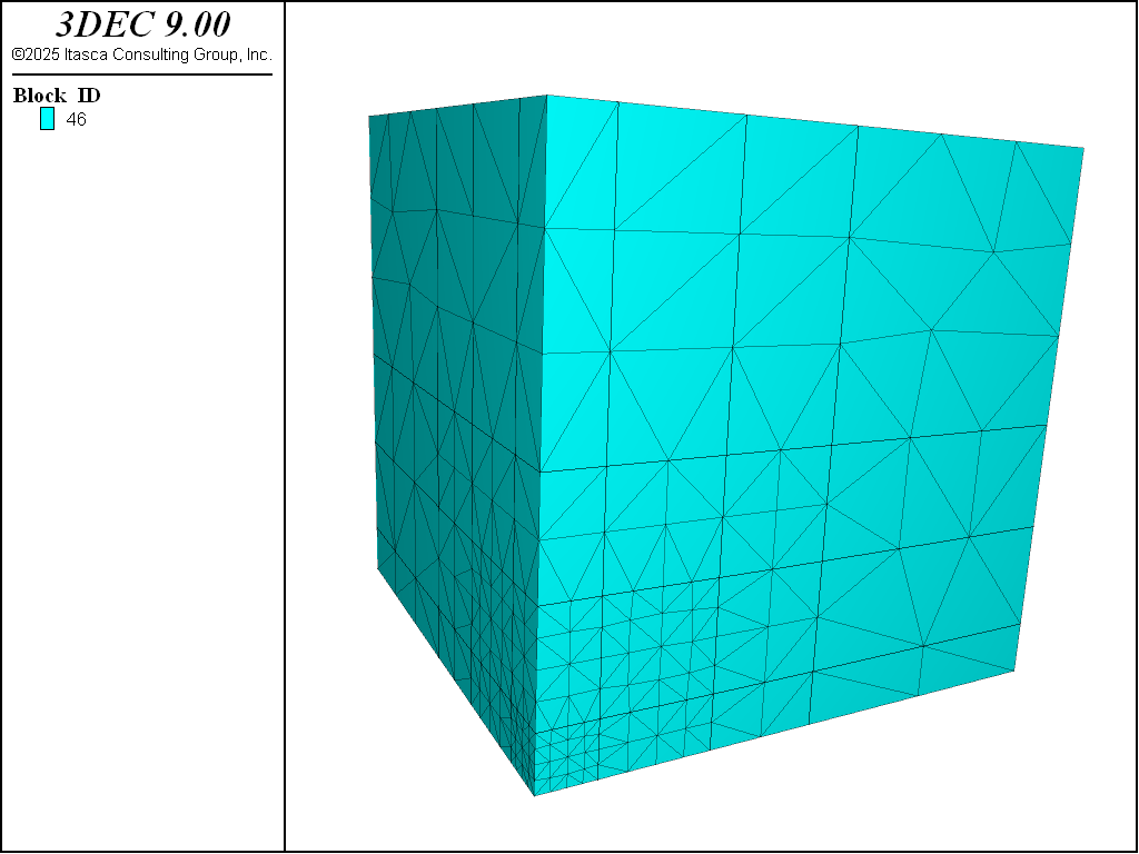
Figure 5: 3DEC model for instantaneous point source.

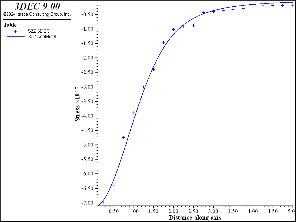
Figure 6: Radial stress (\(S_{zz}\)) on \(z\)-axis (\(x = y\) = 0) after 1 and 3 days.
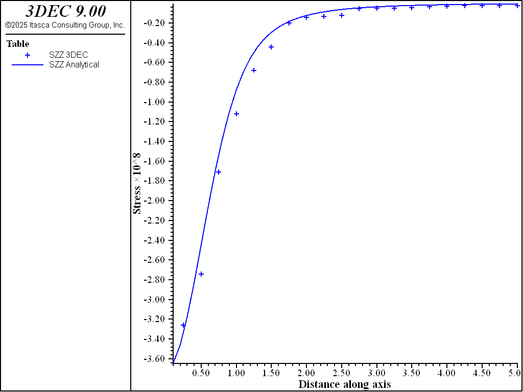
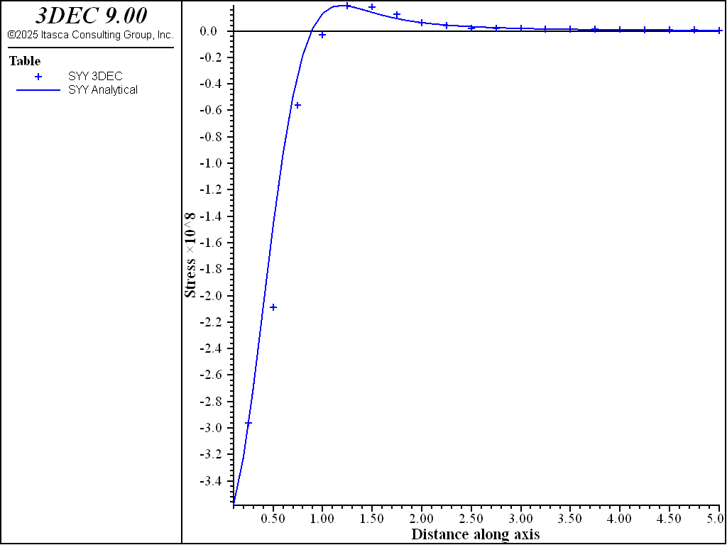
Figure 7: Tangential stresses \(S_{xx}\) and \(S_{yy}\) along \(z\)-axis (\(x = y\) = 0) after 1 day.

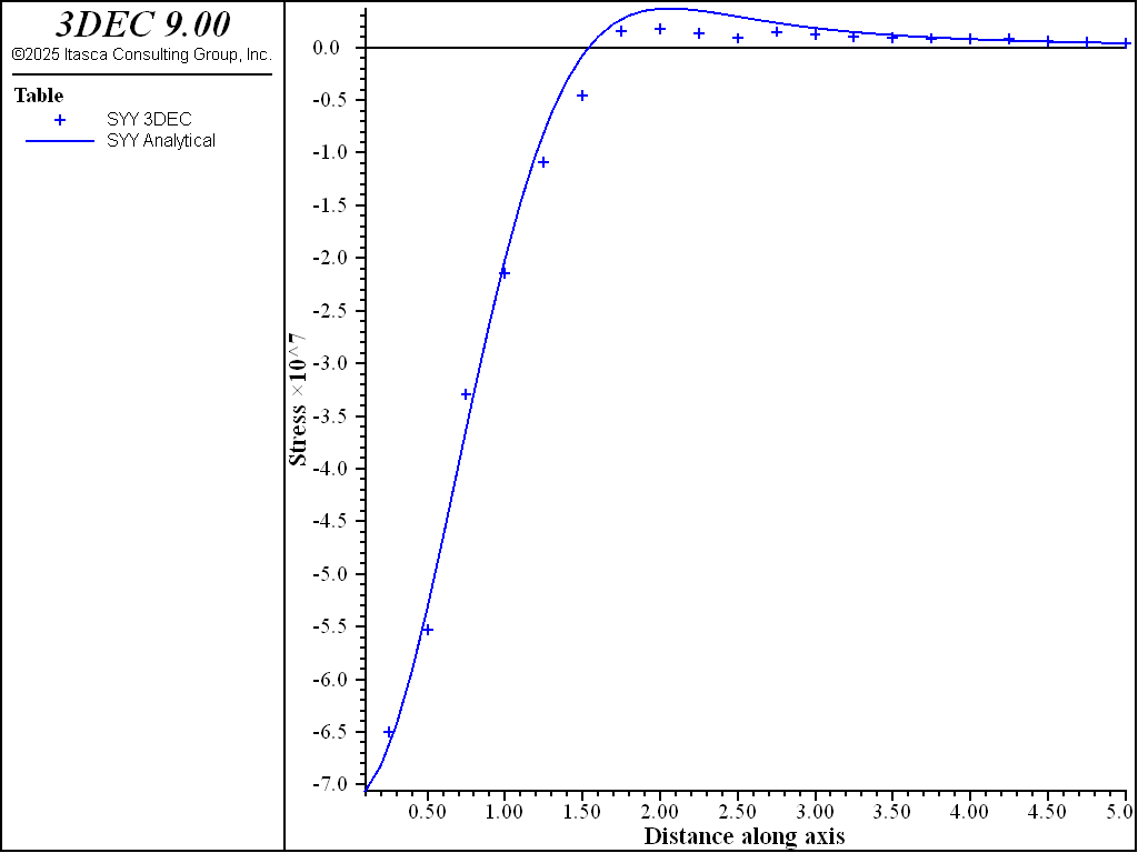
Figure 8: Tangential stresses \(S_{xx}\) and \(S_{yy}\) along \(z\)-axis (\(x = y\) = 0) after 3 days.
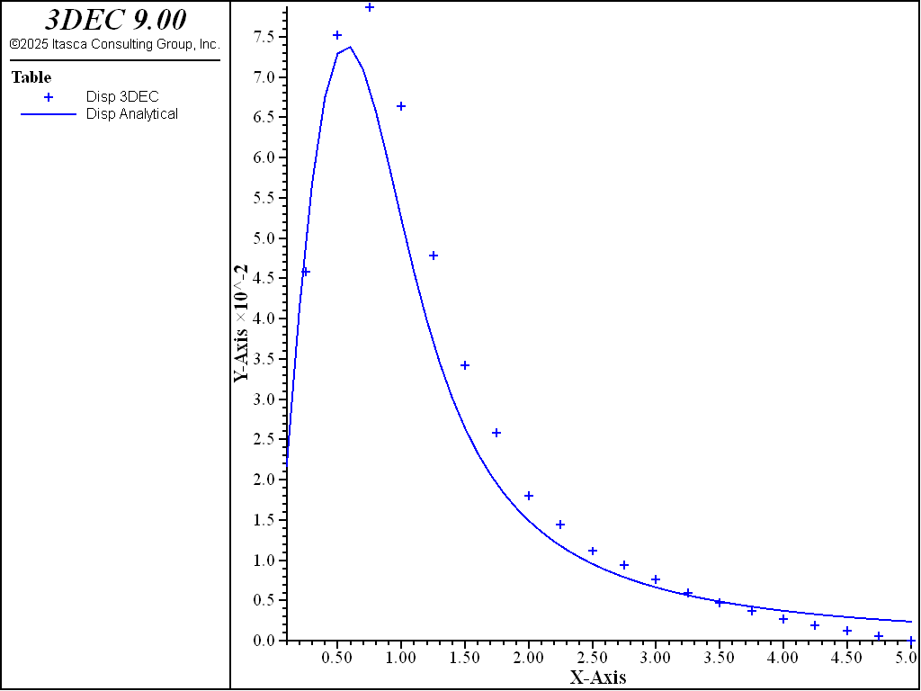
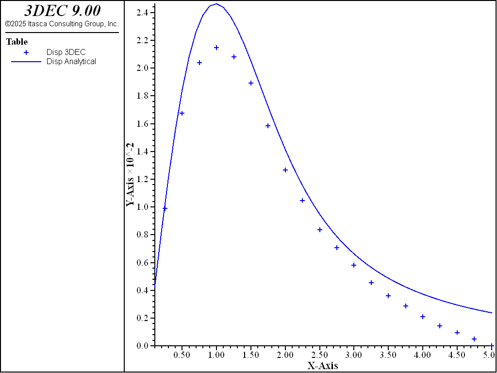
Figure 9: \(z\)-displacement along \(z\)-axis after 1 and 3 days.
An Example Problem – Waste Repository Drift Model
Figure 11 shows a cross section through a drift in a hypothetical nuclear waste repository. A heat source in the floor of the drift represents a waste canister. The properties of the host rock are:
thermal conductivity |
2.2 W/m/°C |
density |
2300 kg/m3 |
specific heat |
900 J/kg/°C |
linear thermal-expansion coefficient |
10 × 10−6/°C |
bulk modulus |
8.3 GPa |
shear modulus |
6.3 GPa |
The initial stress is hydrostatic at 5 MPa, and the heat source is assumed to have only one component with a decay constant of 4 × 10⁻¹⁰ s−1 and an initial strength of 30 kW.
For this example, it is assumed that there are other heat sources (spaced 15 m apart along the length of the drift), and that there are other drifts (spaced 20 m apart), also with heat sources in the floor. The mechanical boundary conditions incorporate this symmetry, but the thermal symmetry is simulated by grids of regularly spaced heat sources. All but one member of each grid are located outside the 3DEC grid.
The data file to solve this problem is given below, and Figure 12 shows a close-up 3DEC plot of the block. Figure 12 shows temperatures and displacements in the model.
The grid of sources can be plotted by creating a scalar for each gridpoint as shown in the FISH file below. The plot is shown in Figure 13
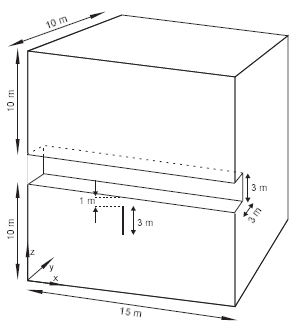
Figure 10: Conceptual model of repository drift.
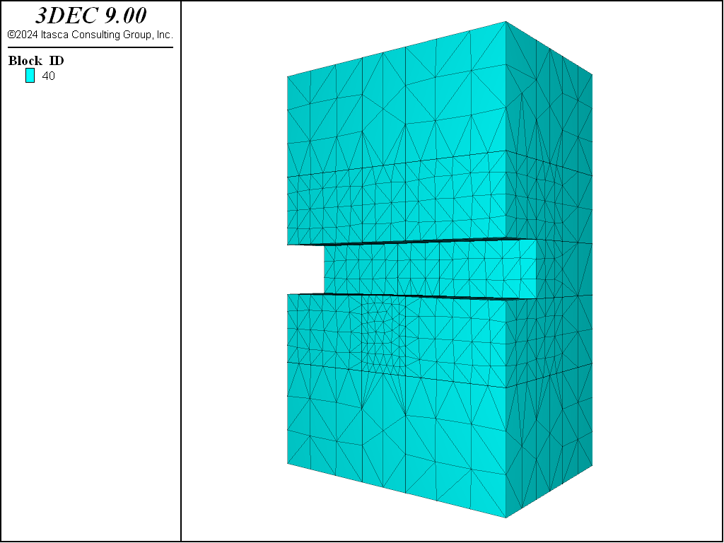
Figure 11: 3DEC model of repository drift.
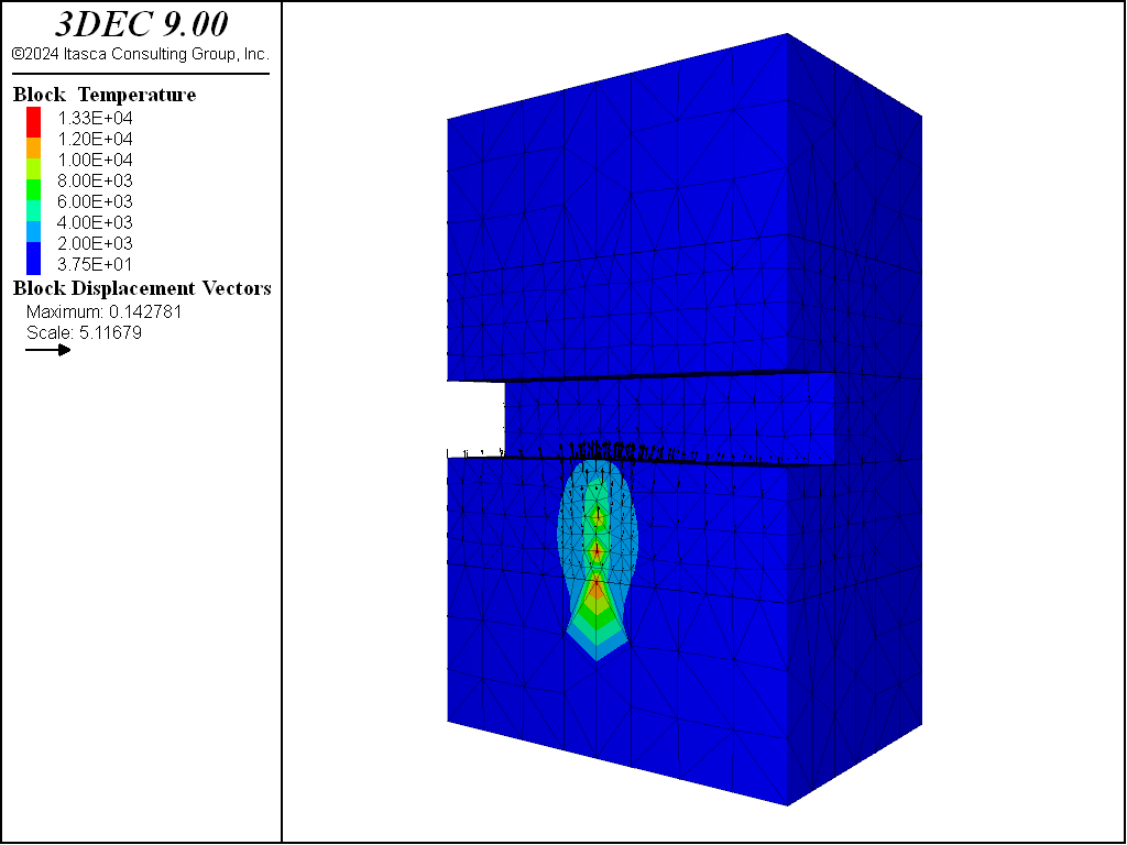
Figure 12: Temperatures and displacements on drift center line.
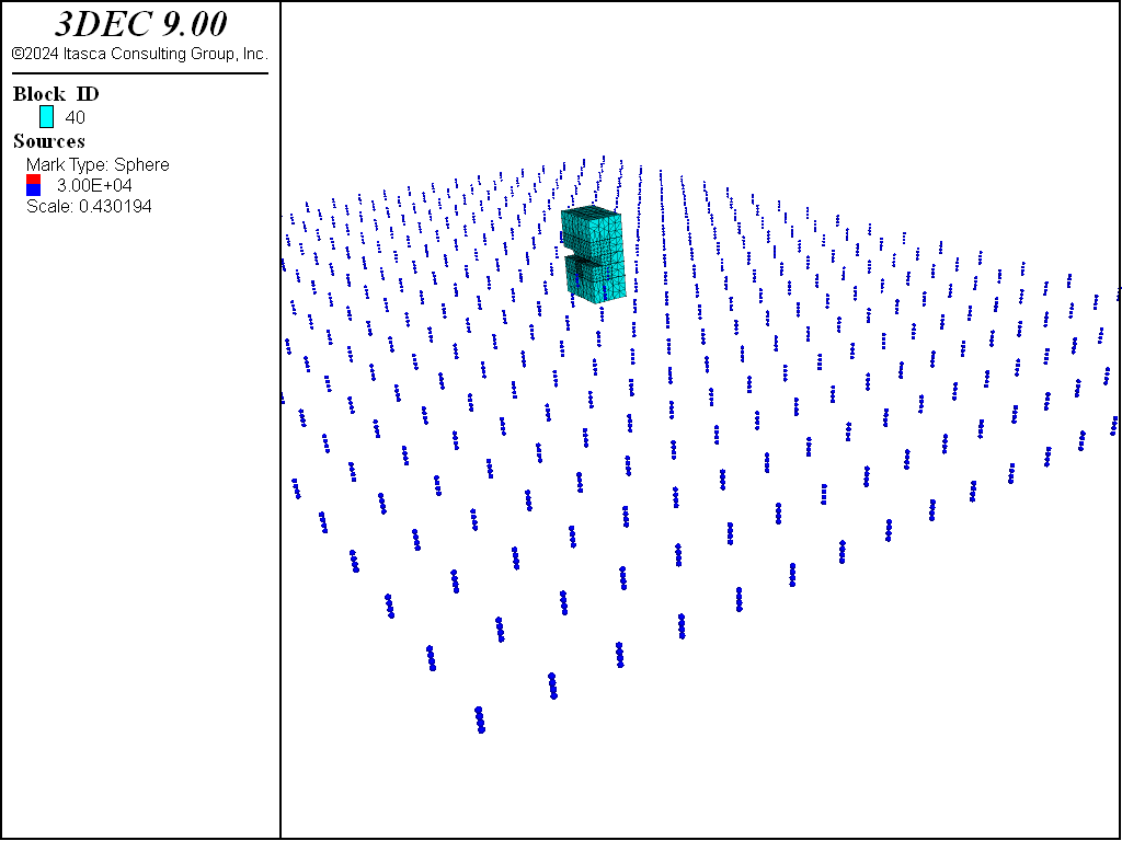
Figure 13: 3DEC model of repository drift with grids of thermal sources.
Data File - AnalyticalDriftdrift.dat
model new
;
; Repository Model
;
model configure thermal
model large-strain on

block thermal analytical on
;
; set up tunnel
;
block create brick 0 15 0 10 0 23
block cut joint-set dip-direction 0 dip 90 origin 0,3,0
block cut joint-set dip-direction 0 dip  0 origin 0,0,13
block cut joint-set dip-direction 0 dip  0 origin 0,0,10
block delete range position-y 0,3 position-z 10,13
;;
;; subdivide forigin mesh refinement
;
block cut joint-set dip-direction 0 dip 90 origin 0.0,6, 0
block cut joint-set dip-direction 0 dip  0 origin 0.0,0, 6
block cut joint-set dip-direction 0 dip  0 origin 0.0,0,17
block cut joint-set dip-direction 90 dip 90 origin 6.,0, 0
block cut joint-set dip-direction 90 dip 90 origin 9.,0, 0
;
; Join all blocks together and zone
;
block join
;
block zone generate edgelength 0.5 ...
  range position-x 6,9  position-y 0,3  position-z 6,10
block zone generate edgelength 1.0 ...
  range position-x 0,15 position-y 0,6  position-z 6,17
block zone generate edgelength 2.0 ...
  range position-x 0,15 position-y 0,10 position-z 0,23
;
model save "repos"
;
; Confine all boundaries to represent symmetry
;
block gridpoint apply velocity-x 0 range position-x 0
block gridpoint apply velocity-x 0 range position-x 15
block gridpoint apply velocity-y 0 range position-y 0
block gridpoint apply velocity-y 0 range position-y 10
block gridpoint apply velocity-z 0 range position-z 0
block gridpoint apply velocity-z 0 range position-z 23
;
block insitu stress -5e6 -5e6 -5e6 0 0 0
;;
block zone cmodel assign elastic
block zone property bulk=8.333e9, shear=6.25e9, density=2300
block zone thermal property expansion=10e-6
block thermal analytical conductivity=2.2 diffusivity=1.1e-6

block contact material-table default property stiffness-normal 1 ...
  stiffness-shear 1
;
;
; Histories
;
block history displacement-z position 7.5,0.4,10.1 ;hist1
;
; Initial equilibrium
;
model solve
model save "repeqm"
;
; After 1 year
;
block thermal source 1 number-components=1, component=1 fraction=1 decay= 4e-10
;
; Define sources to represent a large area around
; modeled drift
;
block thermal grid point-1 -142.5,100,9 point-2 157.5,100,9 ...
                   point-3 157.5,-100,9 source 1 n12=21 n23=21 strength=30e3
block thermal grid point-1 -142.5,100,8 point-2 157.5,100,8 ...
                   point-3 157.5,-100,8 source 1 n12=21 n23=21 strength=30e3
block thermal grid point-1 -142.5,100,7 point-2 157.5,100,7 ...
                   point-3 157.5,-100,7 source 1 n12=21 n23=21 strength=30e3
block thermal grid point-1 -142.5,100,6 point-2 157.5,100,6 ...
                   point-3 157.5,-100,6 source 1 n12=21 n23=21 strength=30e3

block thermal analytical solve time 3.1536e7
model solve

program call 'plotgrid.fis'

model save "repyr1"
Data File - AnalyticalDriftplotgrid.fis
fish define plotgrid
  ; loop through grids
  loop local grid (1,block.thermal.grid.num)
    p1 = block.thermal.grid.point(grid,1) ; top left
    p2 = block.thermal.grid.point(grid,2) ; top right
    p3 = block.thermal.grid.point(grid,3) ; bottom right

    ; make a scalar for each point in the grid with a value equal to the strength
    ; assume each grid lines in the xy plane
    numx = block.thermal.grid.n12(grid)
    numy = block.thermal.grid.n23(grid)
    zpos = p1->z
    loop i (1,numx)
      xpos = p1->x + (p2->x - p1->x)*i/numx
      loop j (1,numy)
        ypos = p2->y + (p3->y - p2->y)*j/numy
        uds = data.scalar.create(xpos,ypos,zpos)
        data.scalar.value(uds) = block.thermal.grid.strength(grid)
      end_loop
    end_loop
  end_loop
end
[plotgrid]
References
Abramowitz, M., and I. A. Stegun. Handbook of Mathematical Functions. New York: Dover Publications Inc. (1972).
Carslaw, H. S., and J. C. Jaeger. Conduction of Heat in Solids, 2nd Ed. Oxford: Clarendon Press (1959).
Crank, J. The Mathematics of Diffusion, 2nd Ed. Oxford: Oxford University Press (1975).
Crouch, S. L., andW. C. McClain. “Interim Report on Development of a Semi-Empirical Numerical Model for Simulating the Deformational Behavior of a High-Level RadioactiveWaste Repository in Bedded Salt,” University of Minnesota Report to Oak Ridge National Laboratory, ORNL/TM-5462 (1978).
Dahlquist, G., and A. Bjorck. Numerical Methods. Englewood Cliffs, New Jersey: Prentice-Hall (1974).
Karlekar, B. V., and R. M. Desmond. Heat Transfer, 2nd Ed. St. Paul: West Publishing Co. (1982).
Nowacki, W. Thermoelasticity. New York: Addison-Wesley (1962).
Perrochet, P., and D. Berod. “Stability of the Standard Crank-Nicolson-Galerkin Scheme Applied to the Diffusion-Convection Equation: Some New Insights,” in Water Resources Research, 29(9), 3291-3297 (September 1993).
| Was this helpful? ... | Itasca Software © 2024, Itasca | Updated: Nov 12, 2025 |
