Adhesive Rolling Resistance Linear Model
The adhesive rolling resistance linear model is based on the rolling resistance linear model, to which an adhesive component is added. It is a linear-based model that can be installed at both ball-ball and ball-facet contacts, and is referred to in commands and FISH by the name arrlinear.
Introduction
A simple cohesive granular material is provided by the adhesive rolling resistance linear model, which is based on the two-dimensional model of [Gilabert2007]. The cohesion arises from a short-range attraction, which is a linear approximation of the van der Waals force law. The short-range attraction differs from the PFC bonded-particle models in that there is no concept of breakage — i.e., the attraction is always present whenever the interacting surfaces come within a specified attraction range. [Gilabert2007] state that assemblies of cohesive grains exhibit much larger variations in their equilibrium densities than do corresponding assemblies of non-cohesive grains, because the cohesive grains may form loose, solid-like cohesive granulates. Such granular systems can stay in mechanical equilibrium at lower solid fractions (down to 25-30%) than cohesionless granular systems (with typical solid fractions of 58-64%). Cohesive granular materials have much less frequently been investigated by numerical simulation than cohesionless ones. The present model encompasses both types of materials, and could be used to study macroscopic behavior of a variety of cohesive granular materials including cohesive powders such as xerographic toners (in which cohesion stems from van der Waals interaction) and wet bead packs (in which cohesion stems from liquid bridges joining neighboring particles). Refer to [Gilabert2007] and [Gilabert2008] for additional information about the structure and mechanical properties of cohesive granular materials as well as additional examples of cohesive packings studied in the laboratory.
Behavior Summary
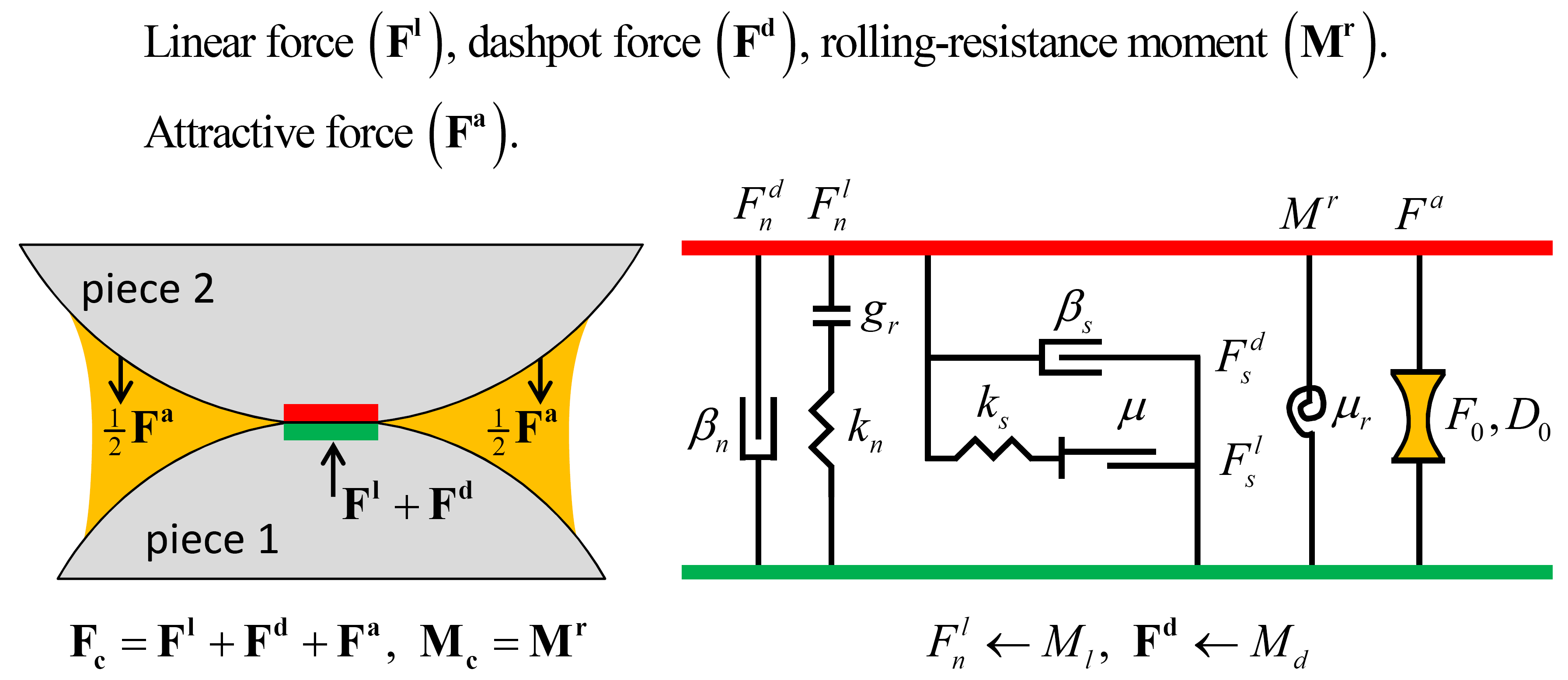
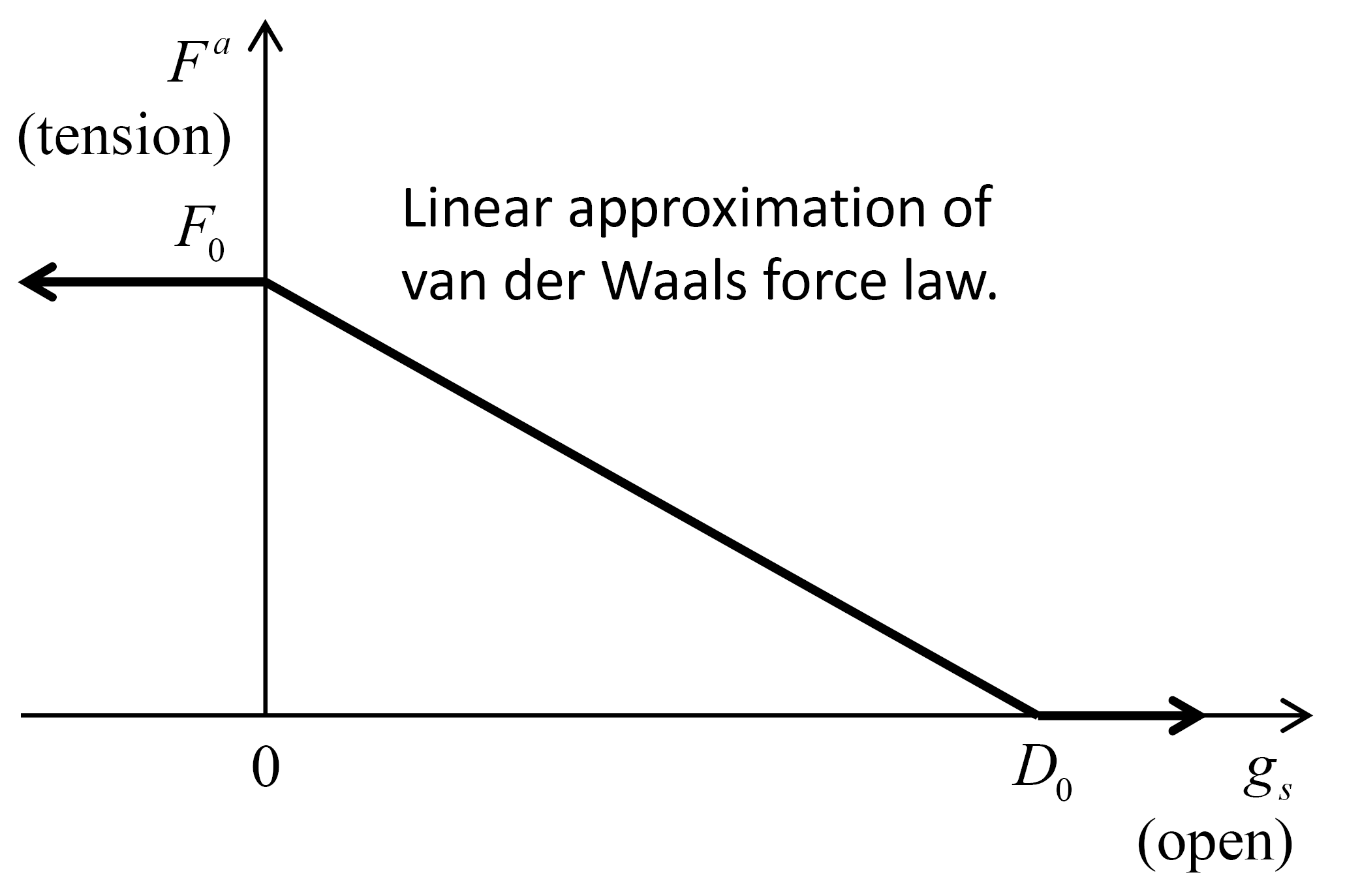
The adhesive rolling resistance linear model provides the behavior of a cohesive granular material via a short-range attraction as a linear approximation of the van der Waals force by adding a cohesive component to the rolling resistance linear model (see Figure 1). The cohesive component is characterized by two parameters: the maximum attractive force \((F_0)\), and the attraction range \((D_0)\) as shown in Figure 2).

Figure 1: Behavior and rheological components of the adhesive rolling resistance linear model. The forces acting on piece 2 are shown, equal and opposite forces act on piece 1.

Figure 2: Attractive force versus surface gap for the adhesive rolling resistance linear model.
Activity-Deletion Criteria
A contact with the adhesive rolling resistance linear model is active if and only if the surface gap is less than the attraction range \((D_0)\). The force-displacement law is skipped for inactive contacts. The surface gap is shown in this figure of the linear formulation. When the reference gap is zero, the notional surfaces coincide with the piece surfaces. If using the CMAT to create an arrlinear material[1], then contacts with the arrlinear model and its associated properties will be created automatically between pieces with a surface gap less than or equal to \(D_0\)[2].
Force-Displacement Law
The force-displacement law for the adhesive rolling resistance linear model updates the contact force and moment as:
where \(\mathbf{F^l}\) is the linear force, \(\mathbf{F^d}\) is the dashpot force, \(\mathbf{F^a}\) is the attractive force, and \(\mathbf{M^r}\) is the rolling resistance moment. The linear force, dashpot force and rolling resistance moment are updated as in the rolling resistance linear model, while the attractive force is updated as follows.
The attractive force acts in the normal direction:
where \(F^a > 0\) is tension (attraction).
Update the attractive force (see Figure 2):
where \(g_s\) is the surface gap.
Energy Partitions
In addition to the energy partitions of the rolling resistance linear model, the adhesive rolling resistance linear model provides the following energy partition:
adhesive energy, \(E_a\), defined as the work done by the attractive force on the contacting pieces.
If energy tracking is activated, this energy partition is updated as follows.
Update the adhesive energy:
(4)\[E_a := E_a - \tfrac{1}{2} \bigl( (F^a)_o + F^a \bigr) \Delta \delta _n\]where \((F^a)_o\) is the attractive force at the beginning of the timestep, and \(\Delta \delta _n\) is the relative normal-displacement increment of Equation (12) of the “Contact Resolution” section. Note that \(E_a\) may be positive or negative, with the convention that work done by the attractive force on the contacting pieces is positive.
Additional information, including the keywords by which these partitions are referred to in commands and FISH, is provided in the table below.
Keyword |
Symbol |
Description |
Range |
Accumulated |
|---|---|---|---|---|
Linear Group: |
||||
|
\(E_{k}\) |
strain energy |
\([0.0,+\infty)\) |
NO |
|
\(E_{\mu}\) |
total energy dissipated by slip |
\((-\infty,0.0]\) |
YES |
Dashpot Group: |
||||
|
\(E_{\beta}\) |
total energy dissipated by dashpots |
\((-\infty,0.0]\) |
YES |
Rolling-Resistance Group: |
||||
|
\(E_{k_r}\) |
rolling strain energy |
\([0.0,+\infty)\) |
NO |
|
\(E_{\mu_r}\) |
total energy dissipated by rolling slip |
\((-\infty,0.0]\) |
YES |
Adhesive Group: |
||||
|
\(E_a\) |
adhesive energy |
\((-\infty,+\infty)\) |
YES |
Properties
The properties defined by the adhesive rolling resistance linear contact model are listed in the table below as a concise reference; see the Contact Properties section for a description of the information in the table columns. The mapping from the surface inheritable properties to the contact model properties is also discussed below.
Keyword |
Symbol |
Description |
Type |
Range |
Default |
Modifiable |
Inheritable |
|---|---|---|---|---|---|---|---|
arrlinear |
Model name |
||||||
Linear Group: |
|||||||
kn |
\(k_n\) |
Normal stiffness [force/length] |
FLT |
\([0.0,+\infty)\) |
0.0 |
YES |
YES |
ks |
\(k_s\) |
Shear stiffness [force/length] |
FLT |
\([0.0,+\infty)\) |
0.0 |
YES |
YES |
fric |
\(\mu\) |
Friction coefficient [-] |
FLT |
\([0.0,+\infty)\) |
0.0 |
YES |
YES |
rgap |
\(g_r\) |
Reference gap [length] |
FLT |
\(\mathbb{R}\) |
0.0 |
YES |
NO |
lin_mode |
\(M_l\) |
Normal-force update mode [-] |
INT |
\(\{0,1\}\) |
0 |
YES |
NO |
\(\;\;\;\;\;\;\begin{cases} \mbox{0: update is absolute} \\ \mbox{1: update is incremental} \end{cases}\) |
|||||||
emod |
\(E^*\) |
Effective modulus [stress] |
FLT |
\([0.0,+\infty)\) |
0.0 |
NO\(^1\) |
N/A |
kratio |
\(\kappa^*\) |
Normal-to-shear stiffness ratio [-] |
FLT |
\([0.0,+\infty)\) |
0.0\(^2\) |
NO\(^1\) |
N/A |
\(\kappa^* \equiv \frac{k_n}{k_s}\) |
|||||||
lin_slip |
\(s\) |
Slip state [-] |
BOOL |
{false,true} |
false |
NO |
N/A |
\(\;\;\;\;\;\;\begin{cases} \mbox{true: slipping} \\ \mbox{false: not slipping} \end{cases}\) |
|||||||
lin_force |
\(\mathbf{F^l}\) |
Linear force (contact plane coord. system) |
VEC |
\(\mathbb{R}^3\) |
\(\mathbf{0}\) |
YES |
NO |
\(\left( -F_n^l,F_{ss}^l,F_{st}^l \right) \quad \left(\mbox{2D model: } F_{ss}^l \equiv 0 \right)\) |
|||||||
user_area |
\(A\) |
Constant area [length*length] |
FLT |
\((0.0,+\infty)\) |
0.0 |
YES |
NO |
Dashpot Group: |
|||||||
dp_nratio |
\(\beta_n\) |
Normal critical damping ratio [-] |
FLT |
\([0.0,1.0]\) |
0.0 |
YES |
NO |
dp_sratio |
\(\beta_s\) |
Shear critical damping ratio [-] |
FLT |
\([0.0,1.0]\) |
0.0 |
YES |
NO |
dp_mode |
\(M_d\) |
Dashpot mode [-] |
INT |
{0,1,2,3} |
0 |
YES |
NO |
\(\;\;\;\;\;\;\begin{cases} \mbox{0: full normal & full shear} \\ \mbox{1: no-tension normal & full shear} \\ \mbox{2: full normal & slip-cut shear} \\ \mbox{3: no-tension normal & slip-cut shear} \end{cases}\) |
|||||||
dp_force |
\(\mathbf{F^d}\) |
Dashpot force (contact plane coord. system) |
VEC |
\(\mathbb{R}^3\) |
\(\mathbf{0}\) |
NO |
NO |
\(\left( -F_n^d,F_{ss}^d,F_{st}^d \right) \quad \left(\mbox{2D model: } F_{ss}^d \equiv 0 \right)\) |
|||||||
Rolling-Resistance Group: |
|||||||
rr_kr |
\(k_r\) |
Rolling resistance stiffness [force*length] |
FLT |
\([0.0,+\infty)\) |
0.0 |
NO |
NO |
rr_fric |
\(\mu_r\) |
Rolling friction coefficient [-] |
FLT |
\([0.0,+\infty)\) |
0.0 |
YES |
YES |
rr_slip |
\(s_r\) |
Rolling slip state [-] |
BOOL |
{false,true} |
false |
NO |
N/A |
rr_moment |
\(\mathbf{M^r}\) |
Rolling resistance moment (contact plane coord. system) |
VEC |
\(\mathbb{R}^3\) |
\(\mathbf{0}\) |
YES |
NO |
\(\left( 0,M_{bs}^r,M_{bt}^r \right) \quad \left(\mbox{2D model: } M_{bt}^r \equiv 0 \right)\) |
|||||||
Adhesive Group: |
|||||||
adh_f0 |
\(F_0\) |
Maximum attractive force [force] |
FLT |
\([0.0,+\infty)\) |
0.0 |
YES |
NO |
adh_d0 |
\(D_0\) |
Attraction range [length] |
FLT |
\([0.0,+\infty)\) |
0.0 |
YES |
NO |
adh_force |
\(F^a\) |
Attractive force \((F^a \ge 0)\) [force] |
FLT |
\([0.0,+\infty)\) |
0.0 |
NO |
NO |
\(^1\) This property is set by the deformability method. |
|||||||
\(^2\) By convention, \(\kappa^* = 0.0\) if either the normal or shear stiffness is 0. |
|||||||
Note
Out-of-balance forces acting on bodies are accumulated during force-displacement calculations. Modifying the forces stored in the contact models will not alter them instantaneously. Therefore, any change to \(\mathbf{F^l}\) may only be effective during the next force-displacement calculation. When \(M_l = 0\), the normal component of the linear force is automatically overridden during the next force-displacement calculation.
Surface Property Inheritance
The linear stiffnesses, \(k_n\) and \(k_s\), and the friction coefficient, \(\mu\), may be inherited from the contacting pieces. See this section from the linear formulation for details. Additionally, the rolling resistance stiffness \(k_r\) is updated if the shear stiffness \(k_s\) is modified.
Methods
The methods of the adhesive rolling resistance linear model are identical to those of the linear model.
Method |
Arguments |
Symbol |
Type |
Range |
Default |
Description |
|---|---|---|---|---|---|---|
area |
Set user_area to the area |
|||||
deformability |
Set deformability |
|||||
emod |
\(E^*\) |
FLT |
\([0.0,+\infty)\) |
N/A |
Effective modulus |
|
kratio |
\(\kappa^*\) |
FLT |
\([0.0,+\infty)^*\) |
N/A |
Normal-to-shear stiffness ratio |
|
\(^*\) By convention, setting \(\kappa^* = 0.0\) sets \(k_s = 0.0\) but does not alter \(k_n\). |
||||||
Area
Set the user_area property via the current contact area. This operation means that the contact area stays constant and is fixed independent of changes to the piece sizes/geometries. In order for the stiffnesses to be recomputed accounting for this area, one should subsequently call the deformabilty method.
Deformability
See this section from the linear formulation for details on these methods.
Callback Events
The callback events defined by the adhesive rolling resistance linear model are identical to those defined by the linear model.
Event |
Array Slot |
Value Type |
Range |
Description |
|---|---|---|---|---|
contact_activated |
Contact has become active |
|||
1 |
C_PNT |
N/A |
Contact pointer |
|
slip_change |
Slip state has changed |
|||
1 |
C_PNT |
N/A |
Contact pointer |
|
2 |
INT |
{0,1} |
Slip change mode |
|
\(\;\;\;\;\;\;\begin{cases} \mbox{0: slip has initiated} \\ \mbox{1: slip has ended} \end{cases}\) |
||||
Usage and Verification Examples
The example Adhesive Rolling Resistance Linear Contact Model: Repose Angle studies the influence of the maximum attractive force on the repose angle of a granular heap.
Model Summary
An alphabetical list of the adhesive rolling resistance linear model methods is given here. An alphabetical list of the adhesive rolling resistance linear model properties is given here.
References
Gilabert, F.A., J.-N. Roux, and A. Castellanos, “Computer Simulation of Model Cohesive Powders: Influence of Assembling Procedure and Contact Laws on Low Consolidation States,” Physical Review E, 75, 011303, 2007.
Gilabert, F.A., J.-N. Roux, and A. Castellanos, “Computer Simulation of Model Cohesive Powders: Plastic Consolidation, Structural Changes and Elasticity under Isotropic Loads,” Physical Review E, 78, 031305, 2008.
Endnotes
| Was this helpful? ... | Itasca Software © 2024, Itasca | Updated: Nov 12, 2025 |
