Elastic Beam with Concentrated Loads

Problem Statement

Note

To view this project in FLAC3D, use the menu command Help ► Examples…. Choose “Structure/Beam/ConcentratedLoadsBeam” and select “ConcentratedLoadsBeam.prj” to load. The data file used is shown at the end of this example.

The maximum midspan deflection, shear-force, and bending-moment distributions for a long thin beam simply supported and loaded by two concentrated loads are computed and compared with the analytical solution for an Euler-Bernoulli beam. This problem quantifies the ability of the Euler-Bernoulli beam element to model the bending action.

Analytical Solution

A simply supported beam of rectangular cross section (of width \((b)\) and depth \((d)\)) is loaded by two equal concentrated loads \((P)\) symmetrically placed. The analytical solution for maximum midspan deflection as well as shear-force and bending-moment distributions corresponds with simple beam theory (Euler-Bernoulli beam theory suitable for long thin beams). The maximum midspan deflection is given by AISC (1980, p. 2-116):

\[\Delta_{\rm max}\ =\ {P a \over {24 E I_z}} \left( 3L^2 - 4 a^2 \right)\]

where \(E\) is Young’s modulus, and \(I_z\) is moment of inertia with respect to \(z\) axis. The analytical solution is for the beam shown in Figure 1.

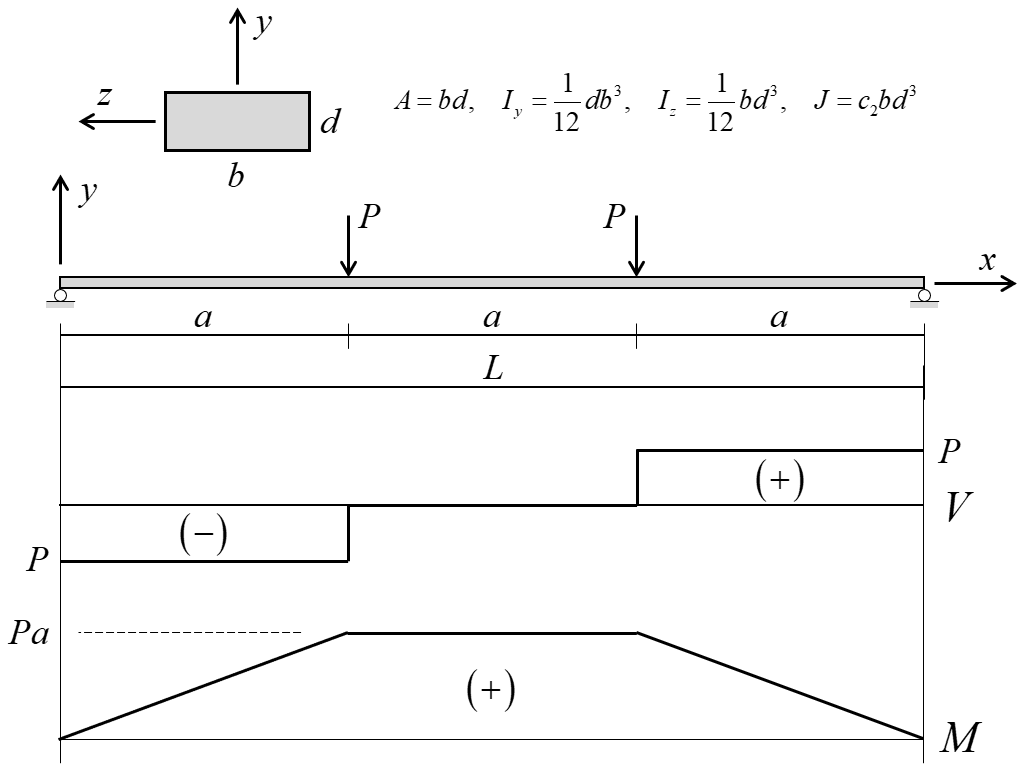
Figure 1: Simply supported beam with two equal concentrated loads and shear-force and bending-moment distributions.

Particular Problem

The particular problem to be considered is defined as follows. The beam has a 9-m length (\(L = 9 \textrm{ m}\) and \(a = 3 \textrm{ m}\)), and a rectangular cross section with \(b = 1.0 \textrm{ m}\) and \(d = 100 \textrm{ mm}\). The cross-sectional properties (obtained via the expressions in Figure 1) are

\[\begin{split}\begin{gather} A = 0.1 \textrm{ m}^2 \\ I_y = 8.33 \times 10^{-3} \textrm{ m}^4, \quad I_z = 8.33 \times 10^{-5} \textrm{ m}^4 \\ J = 3.12 \times 10^{-4} \textrm{ m}^4 \end{gather}\end{split}\]

where the constant \(c_2 = 0.312\) (Crandall et al., 1978, Table 6.1). The beam is comprised of structural steel, and is assumed to behave as an isotropic elastic material with

\[E = 200 \textrm{ GPa}, \quad \nu = 0.30\]

The properties \(\{ A, I_y, J, \nu \}\) are not relevant for this problem; however, they are needed as input for the FLAC3D model. The concentrated loads \((P = 1 \times 10^4 \textrm{ N})\) are applied at the beam third points. For these properties, the maximum midspan deflection is \(15.5312 \textrm{ mm}\).

FLAC3D Model

The FLAC3D model consists of 10 beam elements and 11 nodes, as shown in Figure 2. The beam is created by issuing three separate structure beam create by-line commands to ensure that nodes will lie exactly at the beam third points. Also, four elements are created in the middle third to ensure that a node will lie at the exact beam center, so that the displacement of this node can be compared with \(\Delta_{\rm max}\). The beam element coordinate system is aligned with the global coordinate system by setting the direction-y property equal to \((0,1,0)\). Simple supports are specified at the beam ends by restricting translation in the \(y\)-direction. Two point loads acting in the negative \(y\)-direction are applied at the beam third points. The \(y\)-displacement at the plate center is monitored as a history. Local nonviscous damping is used with a damping factor of 0.8. The model is run in small-strain mode to correspond with the small-strain assumption of the analytical solution. The model is cycled until a convergence limit of \(1 \times 10^{-3}\) is achieved.

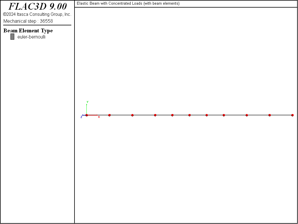
Figure 2: Geometry of the FLAC3D model showing mesh with nodes and global coordinate system.

Results and Discussion

The deformed shape and center-deflection history are shown in Figure 3, from which we conclude that the static solution has been obtained. The maximum deflection occurs at the center and equals \(15.5312 \textrm{ mm}\), which corresponds exactly with the analytical solution. The displacement field in Figure 3 is visualized using the Structural Elements:Beam plot item, checking the Def-Fac box, and assigning a deformation factor of 50. The displacement field can also be visualized as displacement vectors (arrows) that emanate from each node via the Structural Elements:Vectors plot item as shown in Figure 4.

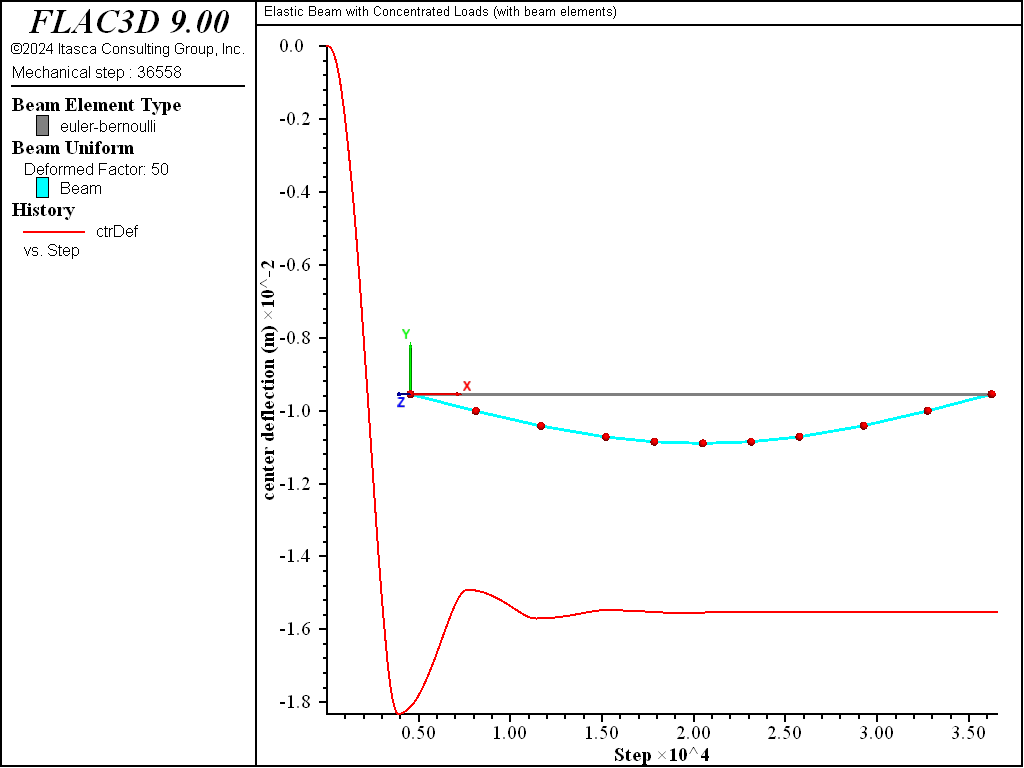
Figure 3: Deformed shape (deformation factor: 50), undeformed shape and center deflection.

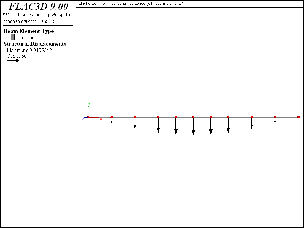
Figure 4: Displacement field plotted as displacement vectors on undeformed shape.

The shear-force and bending-moment distributions are shown in Figures 5 and 6. These distributions correspond exactly with the analytical solution. The quantities are displayed using the force-moment sign convention.

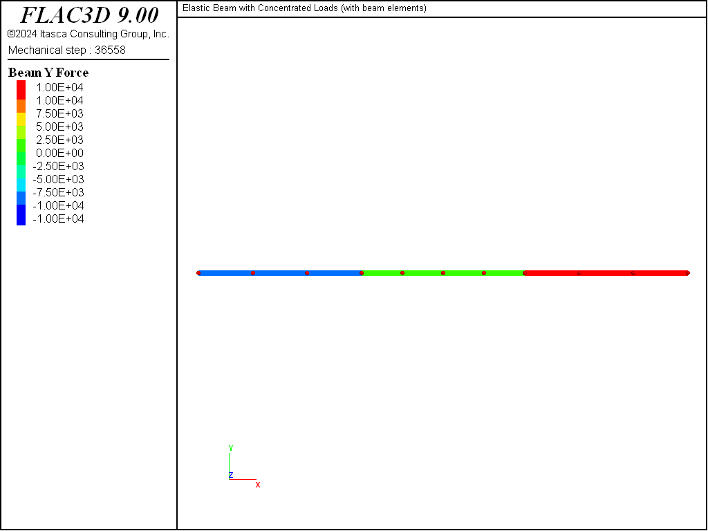
Figure 5: Shear-force distribution (element coordinate system is aligned with global coordinate system).

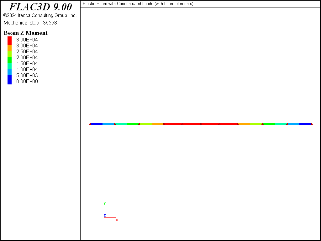
Figure 6: Bending-moment distribution (element coordinate system is aligned with global coordinate system).

The evolution of bending moment at \(x = 1\) is shown in Figure 7 to reach a steady-state value of \(1 \times 10^4 \textrm{ Nm}\). In this plot, we overlay two histories: one has sampled the moment acting at the right end of element 1 and the other has sampled the moment acting at the left end of element 2. If expressed in a consistent system, these two values should be identical, and the plot demonstrates that they are. This is the case, because the elements making up the beam have a consistent orientation (having been created using the structure beam create command). Note that if we list the moment acting on each element in terms of the global system \((M_z)\) with the command

structure beam list force-node global range component-id 1 2

then we find that the moment acting on the right end of element 1 is positive, while the moment acting on the left end of element 2 is negative. This is the correct behavior that satisfies static equilibrium.

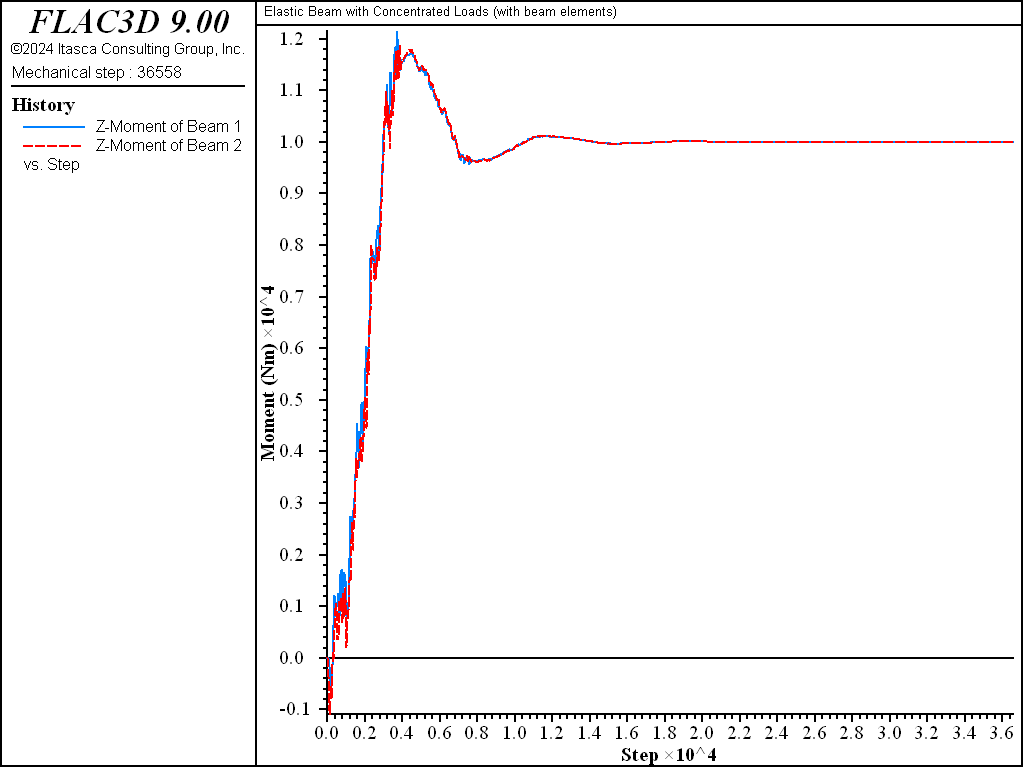
Figure 7: Evolution of bending moment at \(x = 1\).

References

AISC. Manual of Steel Construction, Eighth Edition. Chicago: American Institute of Steel Construction Inc. (1980).

Crandall, S.H., N.C. Dahl and T.J. Lardner. An Introduction to the Mechanics of Solids, Second Edition, New York: McGraw-Hill Book Company (1978).

Data File

ConcentratedLoadsBeam.dat

model new
model title 'Elastic Beam with Concentrated Loads (with beam elements)'

; Create the beam, ensuring that nodes will exist at the third points.
structure beam create by-line ( 0, 0, 0) ( 3, 0, 0) id 1 segments 3 ...
                   element-type euler-bernoulli
structure beam create by-line ( 3, 0, 0) ( 6, 0, 0) id 1 segments 4 ...
                   element-type euler-bernoulli
structure beam create by-line ( 6, 0, 0) ( 9, 0, 0) id 1 segments 3 ...
                   element-type euler-bernoulli

; Assign beam properties.
structure beam cmodel assign elastic
structure beam property young 200e9 poisson 0.30
structure beam property cross-sectional-area 0.1 ...
                     moi-y 8.33e-3 moi-z 8.33e-5 torsion-constant 3.12e-4 ...
                     direction-y (0,1,0)

; Specify boundary conditions (including applied loads).
structure node fix velocity-y range union position-x=0 position-x 9.0
                   ;  rollers at beam ends
structure node apply force (0,-1e4,0) range position-x 3.0 position-x 6.0 union
                   ; apply pointloads

; Setup histories for monitoring behavior.
structure node history name 'ctrDef' displacement-y position (4.5, 0, 0)
structure beam history name 'mom1' moment-z end 2 position (0.5, 0, 0)
                   ; moment, right end of element 1
structure beam history name 'mom2' moment-z end 1 position (1.5, 0, 0)
                   ;  moment, left end of element 2

model large-strain off
structure mechanical damping local 0.8
model solve convergence 1e-3
model save 'ConcentratedLoadsBeam'