FLAC3D Modeling • Problem Solving with FLAC3D
Working with Geometric Data
the program has the capability to import and define arbitrary geometric data. For instance, CAD data from AutoCAD can be imported from a DXF file. This geometry information can be manipulated after creation, and it can also be used for reference in visualization. There are certain (as yet somewhat limited) commands that allow zones or building blocks to be generated from polygons forming a closed volume. In addition, the data can be used to filter the objects affected by a the program command and to identify objects in certain regions by assigning group names.
This section provides a high-level description of how geometric data can be used in the current version of the program. For details, including all available options, see the documentation of commands related to geometric data in the c geometry commands.
The data files and geometry data used to generate all the images in this section can be found in the project UsersGuide\\ProblemSolving\\GeometricData\\GeometricData.prj in the datafiles folder of the the program distribution.
Note that a discussion of using geometric data to create densified “octree” grids can be found in Grid Generation in FLAC3D under Geometry-Based Densification: Octree Meshing.
The data files and geometry data used to generate all the images in this section can be found in the project Users_Guide\\geometry\\geometry.prj in the datafiles folder of the 3DEC distribution.
Note that a discussion of generating block assemblies from geometric surfaces can be found in Generating Block Assemblies. Cutting blocks with geometries is described in Cutting Blocks and finally, using geometric data to create densified “octree” grids is described in in Block Generation: Densify and Octree.
Geometric Data
the program organizes geometric data into sets, which are named collections of polygons, edges, and nodes. The data are topologically connected. Polygons are defined by a series of edges, and edges are defined by two nodes.
The easiest way to create a geometric set is via the geometry import command. For example, the command
geometry import 'surface1.stl'
will import the data in the file surface1.stl and place it into a geometric set called surface1. Currently available formats are DXF, STL, and an Itasca-defined format that preserves added metadata (e.g., group names, FISH extra variables, etc.). You can also simply go to the menu command (Ctrl + O) and select a geometry file with a recognized extension (STL, DXF, and GEOM) in the ensuing dialog.
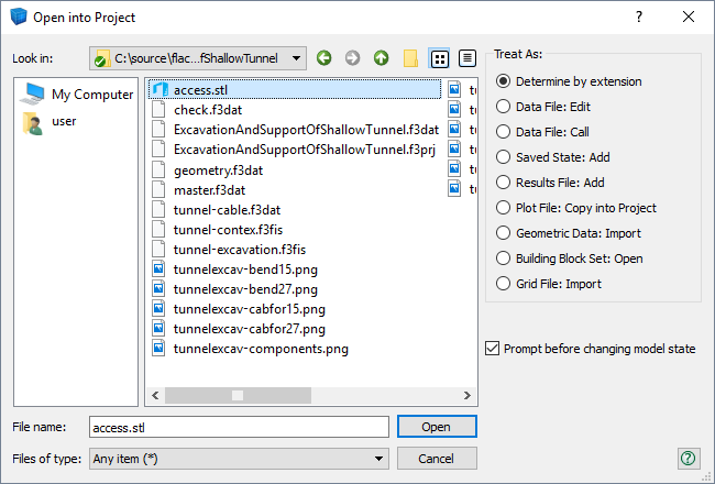
Figure 1: The the program Open into Project dialog.
Geometric data can also be created via commands. For instance, the geometry polygon create command
can be used to directly add a polygon to a geometric set. For example,
geometry polygon create by-positions (0,0,0) (1,0,0) (1,1,0) (0,1,0)
will add a simple quadrilateral to the current geometry set.
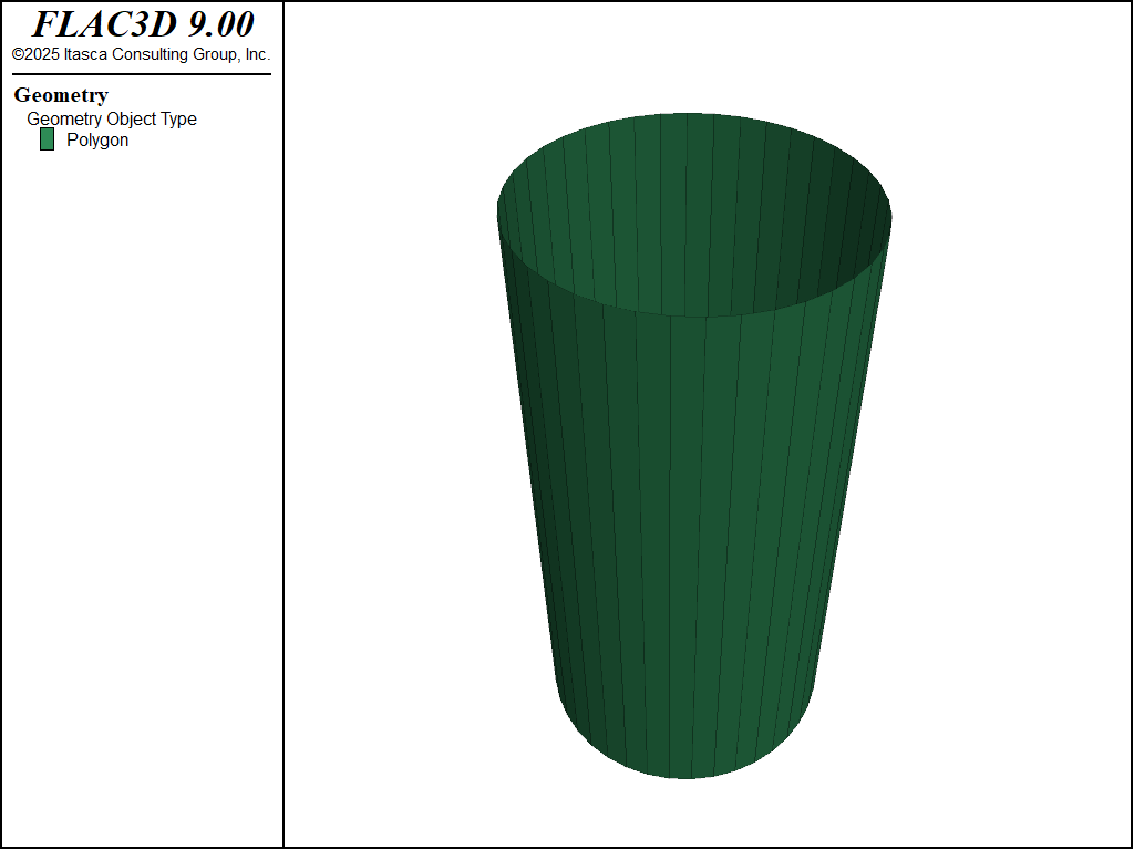
In addition, all data in all sets are available through FISH (see the topic Geometry FISH Functions for a list of functions). FISH can be used to both modify and create geometric data. For instance, the following is a simple FISH function that creates a geometric set called “FISH Example” and then adds polygons forming a cylinder:
Example: “fish_cylinder.fis”
model new
fish define fish_cylinder(start,radius,height,segments)
    local gset = geom.set.find("FISH Example")
    if gset = null then
        gset = geom.set.create("FISH Example")
    endif
    loop local i (1,segments)
        local ang1 = float(i-1) * math.pi * 2.0 / float(segments)
        local ang2 = float(i)   * math.pi * 2.0 / float(segments)
        local p1 = start + vector(math.cos(ang1),math.sin(ang1),0.0)
        local p2 = start + vector(math.cos(ang2),math.sin(ang2),0.0)
        local p3 = vector(p2->x,p2->y,height)
        local p4 = vector(p1->x,p1->y,height)
        local poly = geom.poly.create(gset)
        geom.poly.add.node(gset,poly,p1)
        geom.poly.add.node(gset,poly,p2)
        geom.poly.add.node(gset,poly,p3)
        geom.poly.add.node(gset,poly,p4)
        geom.poly.close(gset,poly)
    end_loop
end
[fish_cylinder((0,0,0),1.0,4.0,40)]
The results are shown below. Following figure has no caption.
Geometry Visualization
Geometric data can be visualized in a i Plot pane. When the dialog is used, the geometry will be automatically rendered in a new plot.
If the set is added by command at the command prompt, it will need to be added manually to a plot to be seen. To do so:
Create a plot ( or Ctrl + Shift + N).
Use the Build Plot tool (
) to get the Build plot dialog, pick the “Geometry” item from the list in the “User Defined Data” category.
In “Attributes”, make sure that the desired set is selected in the “Sets” control. (Note: With this control, more than one set maybe visualized on the same plot item.)
Geometry Painting
To help visualize how model variables vary with respect to geometry data, data from the zones can be used to “paint” values on to geometric nodes. These values can then be contoured to visualize how model variables vary in relation to geometric features that might not be explicitly modeled.
By switching the “Type” attribute to “Contour”, and switching the “ContourBy” value to “FieldData”, you can select from the list of all zone field variables. This data is used only for plotting, and is not visible to the model state.
The geometry paint-extra command, however, can be used to “paint” zone field data values
from the model to an extra variable stored in geometric nodes. For example, to paint the minimum
principal stress in the model onto the active geometric set, you use the command
geometry paint-extra 2 stress quantity minimum
which will calculate minimum principal stresses at the location of all nodes in the active set,
and assign that value to extra variable index 2. The complete list of zone field variables
available can be found in the geometry paint-extra command documentation.
The result of painting can be visualized by using the Geometry plot item (with attributes “Type” = “Contour”, “Contour By” = “Node Extra”, and “Index” = “2”). The figure below is an example of painting the displacement magnitudes on a simple tunnel next to the main excavation.
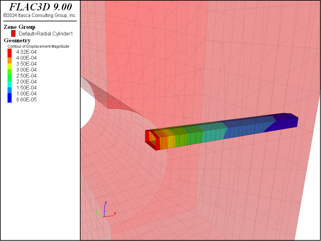
Figure 3: Displacement magnitude painted on geometry.
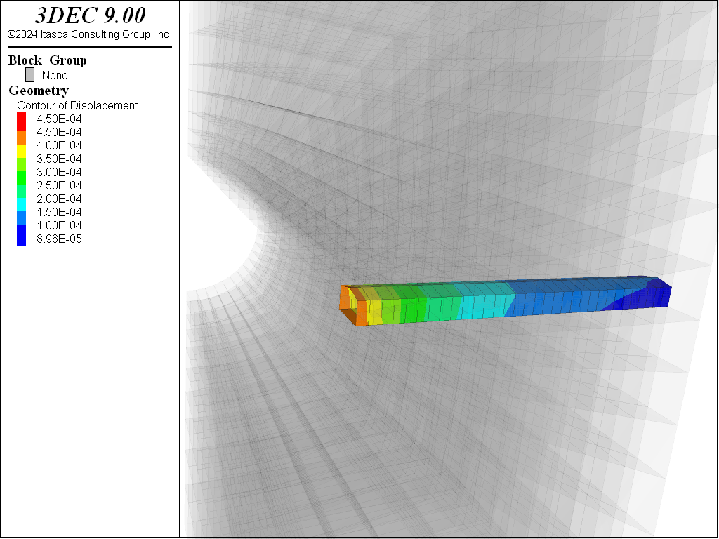
Figure 4: Displacement magnitude painted on geometry.
Geometric Filtering - Geometry Range Elements
The primary method for selecting objects in FLAC3D is to provide a filter that determines the objects affected by a given command. This is done using the range logic. There are two range elements that exist to filter objects based on their relation to data in geometric sets: geometry-distance and geometry-space.
The geometry-distance range element can be used to select objects that fall within a given distance of data in a geometric set. This includes polygons, free edges and free nodes. The minimum distance from the object centroid to any data in the set determines the distance value.
The extent keyword is valid for the geometry-distance range element, finding the minimum distance to the Cartesian extent of an object. This can be used with a distance value of zero to return an approximation of all objects that actually intersect the geometric set. For example, the following command can be used with the above data to assign group name “Intersect” to all zones blocks that have a Cartesian extent that intersects the geometric set “intcylinder.”
zone group "Intersect" range geometry-distance "intcylinder" gap 0.0 extent
The result of that operation is shown here.
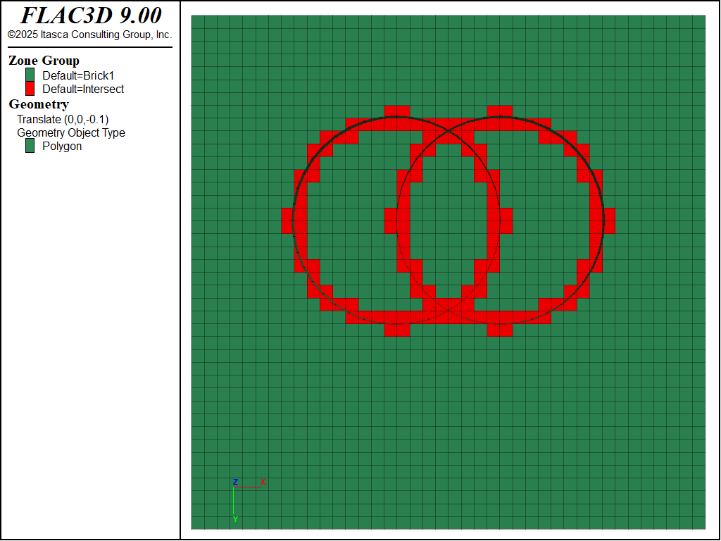
Figure 5: Zones selected by the geometry dist range element.
block group 'Intersect' range geometry-distance 'intcylinder' gap 0.0 extent
The result of that operation is shown here.
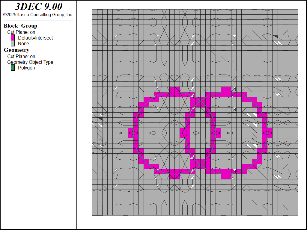
Figure 6: Blocks selected by the geometry dist range element.
The geometry-space range element selects objects based on how many times a ray starting from the object intersects polygons from the geometric set. If the intersection count matches the number provided, it is considered selected. This can be used to identify objects above or below a geometric surface (e.g., topography).
In the example below, a ray is projected in the positive x-direction and all objects inside of the right-hand cylinder are selected since a ray projected from the centroid only hits the cylinder one time.
zone group "Count 1" range geometry-space "intcylinder" ...
                           count 1 direction (1,0,0)
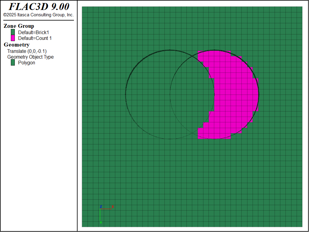
Figure 7: Zones selected by the geometry count range element.
block group 'Count 1' range geometry-space 'intcylinder' ...
  count 1 direction 1 0 0
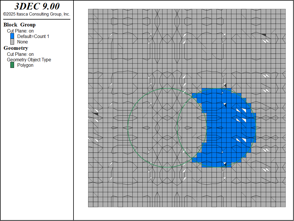
Figure 8: Blocks selected by the geometry count range element.
As a special case, the keywords odd or even can be substituted in place of a count number in the geometry count range element. If the geometric set effectively forms a closed volume, the odd keyword will result in selecting all objects inside, and the even will select all objects outside. No checking is done to make certain the polygons actually form a single closed surface. The results of the command
zone group "Count Odd" range geometry-space "intcylinder" ...
                             count odd direction (1,0,0)
block group 'Inside' range geometry-space 'intcylinder' ...
  count odd direction 1 0 0
are shown in in the next figure. Note that the intersecting cylinder geometry set does not form a single closed surface, and therefore, the range element does not select zones in the shared region.
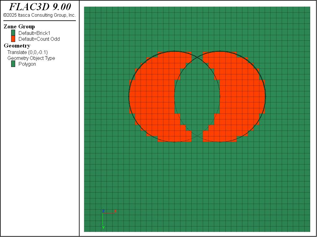
Figure 9: Zones selected by the geometry count range element using the odd keyword.
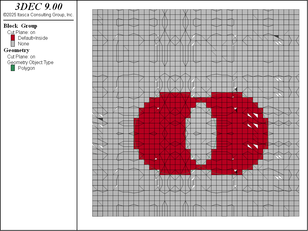
Figure 10: Blocks selected by the geometry count range element using the odd keyword.
If the geometric set does form a perfect topologically closed volume, then the inside and outside keywords can be used to select objects instead of the count keyword.
Geometry Data and Group Assignment
There are occasions when you wish to select objects that fall into regions of space delineated by complex geometric data. Sometimes these data are not neatly separated into distinct surfaces that can be assigned to different geometric sets. Sometimes the relation between the data is complex, and manually identifying specific regions (e.g., above this surface, behind that, and ahead of this) is burdensome. The geometry assign-groups command lets you assign group names to objects based on how they relate to all these surfaces at once.
The operation works by first assigning a unique ID number to all polygons that form a single contiguous surface. Specifically, all polygons in a single set that are connected across edges will be given the same ID number. A ray is then passed from the centroid of the object through those polygons, and a group name is generated based on how many times the ray intersects polygons of each ID.
As a simple example, we will use a geometric set consisting of two intersecting cylinders. The
geometry assign-groups command is used to assign group names to objects based on their relation to the
surfaces using the command
geometry assign-groups zone projection (1,0,0) set 'intcylinder'
geometry assign-groups block projection (1,0,0) set 'intcylinder'
The figure below shows the group name assigned to zones in a cut-plane through the model. Each letter represents a different intersection region as defined by surface ID and intersection count.
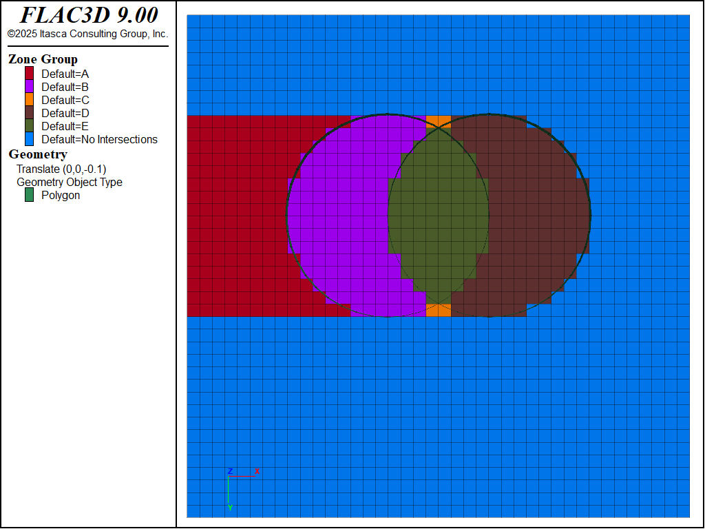
Figure 11: Groups assigned by the geometry assign-groups command.
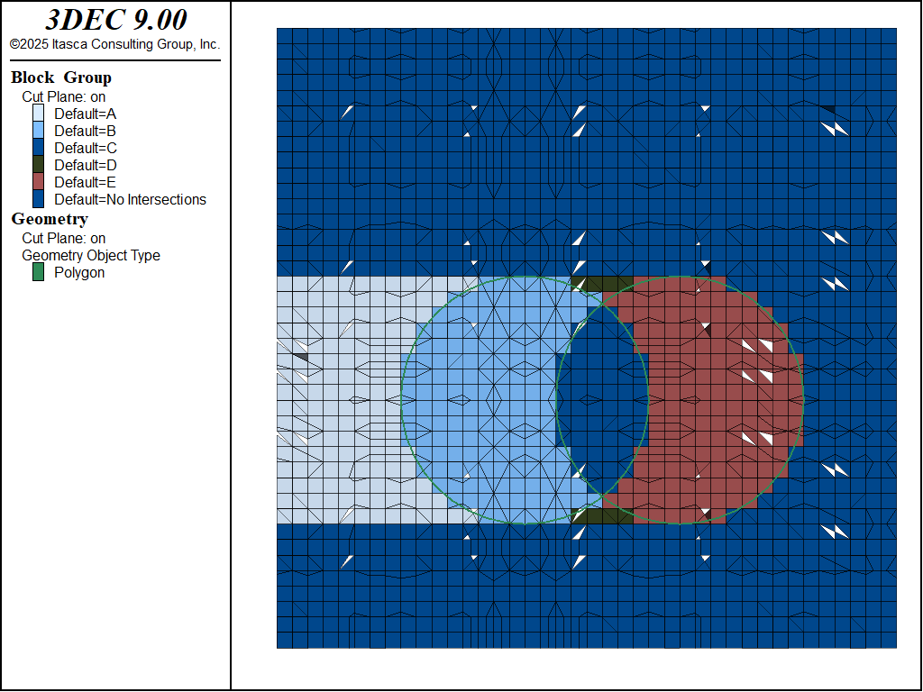
Figure 12: Groups assigned by the geometry assign-groups command.
This operation may be performed on virtually any object including zones, gridpoints, user-defined data and structural element objects (elements, nodes, and links).
While the geometry assign-groups command can quickly separate objects into separate geometric regions, it does have limitations. The user has no control over the ID numbers assigned to surfaces, and determining the group names assigned to desired regions has to be done via visual inspection. Often, multiple groups will need to be combined into the actual region of interest.
Geometry Data: Examples
Geometry data can be used for a variety of zone-generation and zone-configuration purposes, including when:
you want to carve groups out of an existing FLAC3D model along several surfaces;
you want, in an existing grid, to assign different groups to zones that will be excavated each year given a number of DXF files representing yearly excavation surfaces;
you want to assign ubiquitous joint properties to zones that come within 10 m of a set of faults; and,
you want to refine a FLAC3D model before identifying a group of zones as weak material.
The examples that follow illustrate the methods available for using geometry data to achieve these purposes.
Title |
|
|---|---|
Example 1 |
Assign Group Names Based on Their Relationship to DXF Files |
Example 2 |
Ignore Existing Groups – Build New Ones Based on Surfaces |
Example 3 |
Partition Existing Groups Based on Surfaces |
Example 4 |
Zones below Surfaces become Separate Groups — Outside Groups Remain Unchanged |
Example 5 |
Zones above the Surfaces become a New Group — Everything below is Unchanged |
Example 6 |
Zones Intersecting Surfaces becomes Separate Groups |
Example 7 |
Split Zones below Surfaces |
Example 8 |
Split Large Zones Intersecting Surfaces |
Assign Group Names Based on Their Relationship to DXF Files
Run FLAC3D and call the following data file, which creates 3 groups called “dummy1,” “dummy2” and “dummy3”:
Example: “Example_1.dat”
;Build a model with 3 groups
model new
zone create brick size (50,50,50) point 0 (2700,-10500,-1000) ...
		               edge 4000 group 'dummy3'
zone delete range position-z 0 1000000
geometry import 's1.dxf'
zone group 'dummy1' ...
           range geometry-space 's1' count 1 direction (0,1,0)
geometry import 's2.dxf'
zone group 'dummy2' ...
           range geometry-space 's2' count 1 direction (1,0,0) group 'dummy3'
Create a plot (Ctrl + Shift + N) and use the “Build Plot” tool ( ) to add zone group surfaces and geometry to the plot. Select the “Zone Group Default” item in the control panel, then set the “Slot” attribute to “Default.” Select the “Geometry Type” item, open the “Sets” attribute, and check the “s2” set; also check the “transparency” box. Click in the plot window to activate it. Press “i” to obtain an axonometric view of the model (as below).
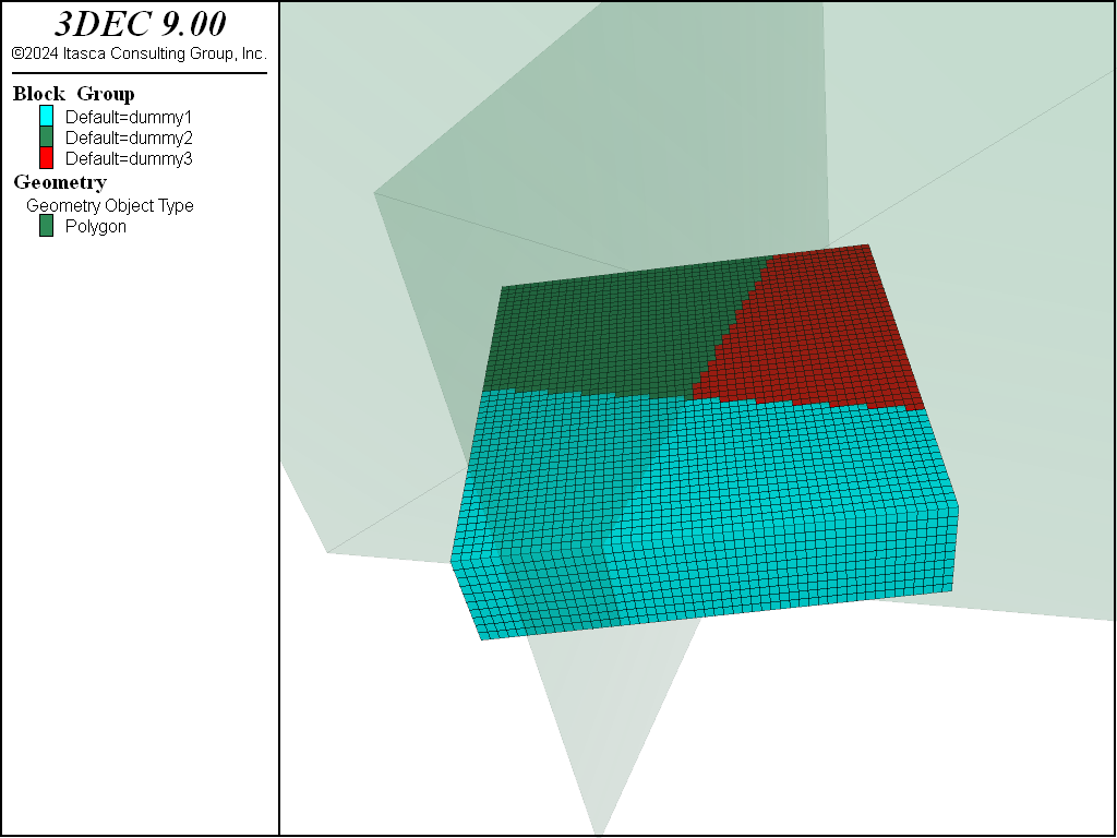
Figure 13: Partitioned model and two surfaces
We will use three surfaces to partition this model into multiple groups, in several different ways. These three surfaces are stored in three separate DXF files called “Y0.dxf,” “Y1.dxf” and “Y2.dxf.” You can think of these surfaces as three excavation surfaces in an open pit mine representing Year0, Year1 and Year2. The next image shows how the model appears when the surfaces are plotted; these DXF files are imported in the next data file example.
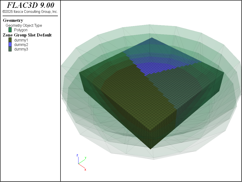
Figure 14: Three surfaces used for partitioning the model with geometry data
Ignore Existing Groups — Build New Ones Based on Surfaces
Existing groups are renamed “old,” and new groups are created based on surfaces (see image below).
Example: “Example_2.dat”
;Ignore existing groups. Build new ones based on surfaces
;(SpaceRanger Option 0)
geometry import 'Y0.dxf'
geometry import 'Y1.dxf'
geometry import 'Y2.dxf'
zone group 'OLD'
zone group 'NEW_1' range geometry-space 'Y0' count odd
zone group 'NEW_2' range geometry-space 'Y1' count odd
zone group 'NEW_3' range geometry-space 'Y2' count odd
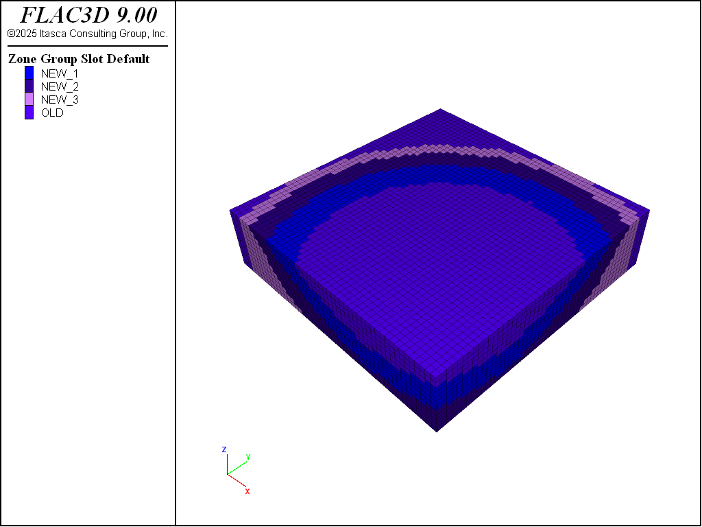
Figure 15: Ignore existing groups — build new ones based on surfaces
Partition Existing Groups Based on Surfaces
Zones outside or above the surfaces maintain their old group number. Zones that are inside or below any of the surfaces are partitioned into new groups along the surfaces (see the figure below).
Example: “Example 3.dat”
;Partition existing groups based on surfaces
; (SpaceRanger Option 1)
model new
zone create brick size (50,50,50) point 0 (2700,-10500,-1000) ...
		               edge 4000 group 'dummy3'
zone delete range position-z 0 1000000;
geometry import 's1.dxf'
zone group 'dummy1' range geometry-space 's1' count 1 direction (0,1,0)
geometry import 's2.dxf'
zone group 'dummy2' ...
           range geometry-space 's2' count 1 direction (1,0,0) group 'dummy3'
geometry import 'Y0.dxf'
geometry import 'Y1.dxf'
geometry import 'Y2.dxf'
zone group 'NEW_1' range geometry-space 'Y0' count odd group 'dummy1'
zone group 'NEW_2' range geometry-space 'Y0' count odd group 'dummy2'
zone group 'NEW_3' range geometry-space 'Y0' count odd group 'dummy3'
zone group 'NEW_4' range geometry-space 'Y1' count odd group 'NEW_1'
zone group 'NEW_5' range geometry-space 'Y1' count odd group 'NEW_2'
zone group 'NEW_6' range geometry-space 'Y1' count odd group 'NEW_3'
zone group 'NEW_7' range geometry-space 'Y2' count odd group 'NEW_4'
zone group 'NEW_8' range geometry-space 'Y2' count odd group 'NEW_5'
zone group 'NEW_9' range geometry-space 'Y2' count odd group 'NEW_6'
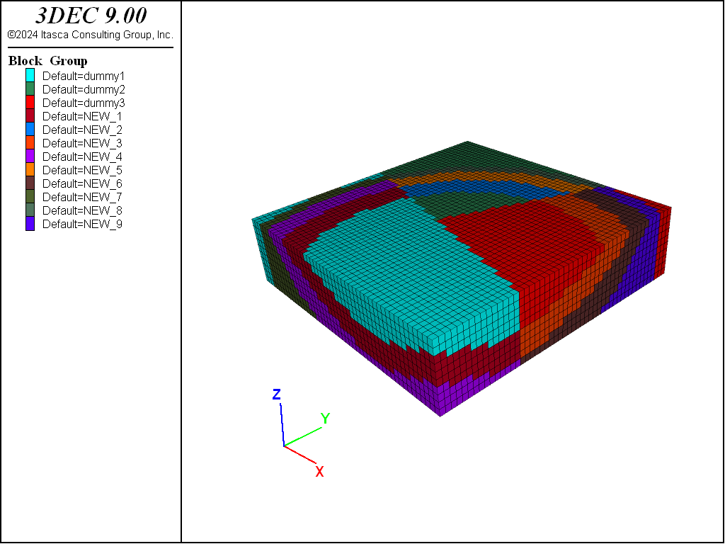
Figure 16: Partitioning everything below surfaces
Zones below Surfaces become Separate Groups, Outside Groups Remain Unchanged
Everything inside or below the surfaces is partitioned. Everything outside or above remains at its original group number (see image below).
;Zones below surfaces become separate groups ...
;  outside groups remain unchanged
;(SpaceRanger Option 2)
model new
zone create brick size (50,50,50) point 0 (2700,-10500,-1000) ...
		               edge 4000 group 'dummy3'
zone delete range position-z 0 1000000
geometry import 's1.dxf'
zone group 'dummy1' range geometry-space 's1' count 1 direction (0,1,0)
geometry import 's2.dxf'
zone group 'dummy2' ...
           range geometry-space 's2' count 1 direction (1,0,0) group 'dummy3'
geometry import 'Y0.dxf'
geometry import 'Y1.dxf'
geometry import 'Y2.dxf'
zone group 'NEW_1' range geometry-space 'Y0' count odd
zone group 'NEW_2' range geometry-space 'Y1' count odd
zone group 'NEW_3' range geometry-space 'Y2' count odd
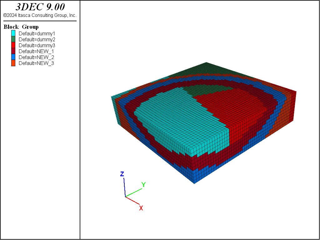
Figure 17: SpaceRanger option 2
Zones above the Surfaces become a New Group, Everything below is Unchanged
Zones above all three surfaces become a new group.
;Zones above surfaces become a new group,
;  everything below is unchanged
;(SpaceRanger option 3)
model new
zone create brick size (50,50,50) point 0 (2700,-10500,-1000) ...
		            edge 4000 group 'dummy3'
zone delete range position-z 0 1000000
geometry import 's1.dxf'
zone group 'dummy1' range geometry-space 's1' count 1 direction (0,1,0)
geometry import 's2.dxf'
zone group 'dummy2' ...
           range geometry-space 's2' count 1 direction (1,0,0) group 'dummy3'
geometry import 'Y0.dxf'
geometry import 'Y1.dxf'
geometry import 'Y2.dxf'
zone group 'NEW_1' range geometry-space 'Y0' count odd not ...
                         geometry-space 'Y1' count odd not ...
                         geometry-space 'Y1' count odd not
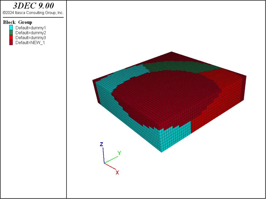
Figure 18: SpaceRanger option 3
Zones Intersecting Surfaces becomes Separate Groups
Zones that intersect the surfaces or come within 80 m of them are grouped as New 1, New 2 and New 3 (see image below).
;Zones intersecting surfaces within 80m become separate groups
;(SpaceRanger option 4)
model new
zone create brick size (50,50,50) point 0 (2700,-10500,-1000) ...
		         edge 4000 group 'dummy3'
zone delete range position-z 0 1000000
geometry import 's1.dxf'
zone group 'dummy1' range geometry-space 's1' count 1 direction (0,1,0)
geometry import 's2.dxf'
zone group 'dummy2' ...
           range geometry-space 's2' count 1 direction (1,0,0) group 'dummy3'
geometry import 'Y0.dxf'
geometry import 'Y1.dxf'
geometry import 'Y2.dxf'
zone group 'NEW_1' range geometry-distance 'Y0' gap 80 extent
zone group 'NEW_2' range geometry-distance 'Y1' gap 80 extent
zone group 'NEW_3' range geometry-distance 'Y2' gap 80 extent
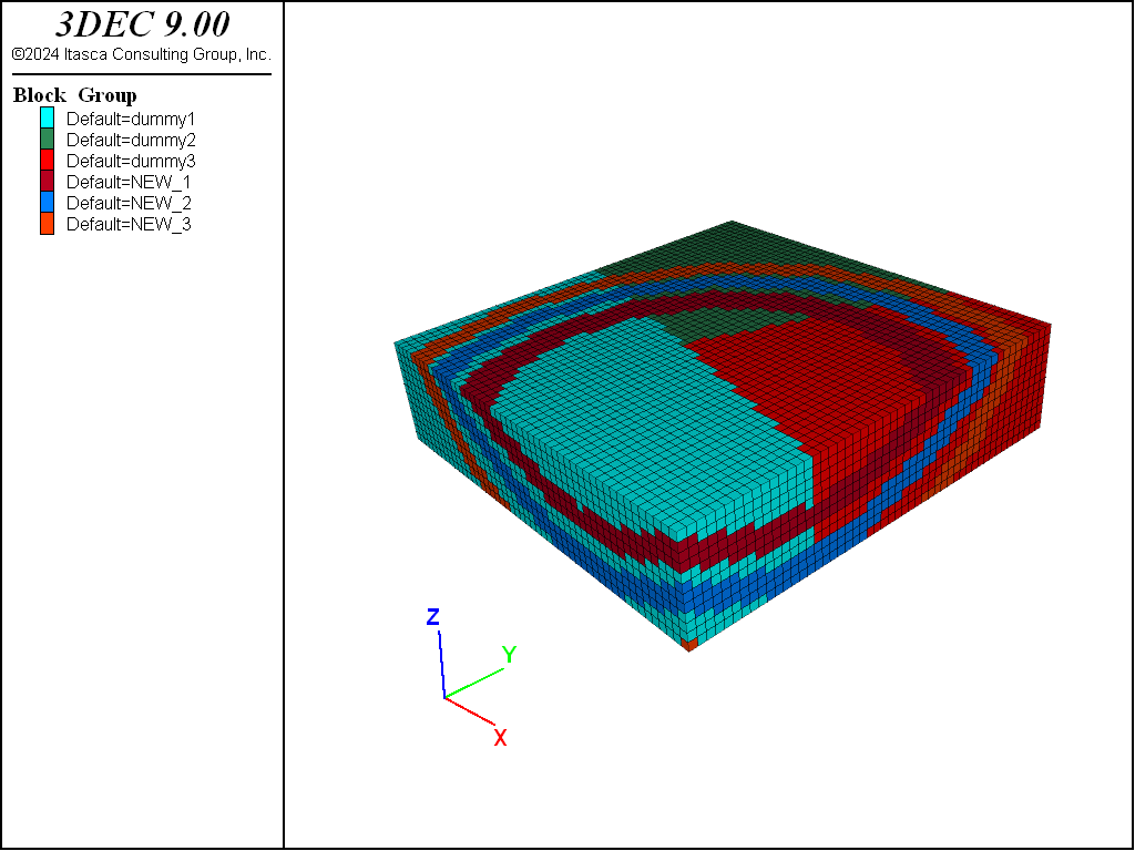
Figure 19: SpaceRanger option 4
Split Zones below Surfaces
Zones below Y0 are refined, then those below Y1, and finally those below Y2 (see image below).
; Split zones below surfaces
; (better than SpaceRanger option 5)
model new
zone create brick size (50,50,50) point 0 (2700,-10500,-1000) ...
		               edge 4000 group 'dummy3'
zone delete range position-z 0 1000000
geometry import 's1.dxf'
zone group 'dummy1' range geometry-space 's1' count 1 direction (0,1,0)
geometry import 's2.dxf'
zone group 'dummy2' ...
           range geometry-space 's2' count 1 direction (1,0,0) group 'dummy3'
geometry import 'Y0.dxf'
geometry import 'Y1.dxf'
geometry import 'Y2.dxf'
zone densify segments 2 range geometry-space 'Y0' count odd
zone densify segments 2 range geometry-space 'Y1' count odd
; The third level of refinement is skipped to keep this model
;    small enough to fit in the 32 bit version.
;generate zone densify nsegment 2 range geometry Y2 count odd
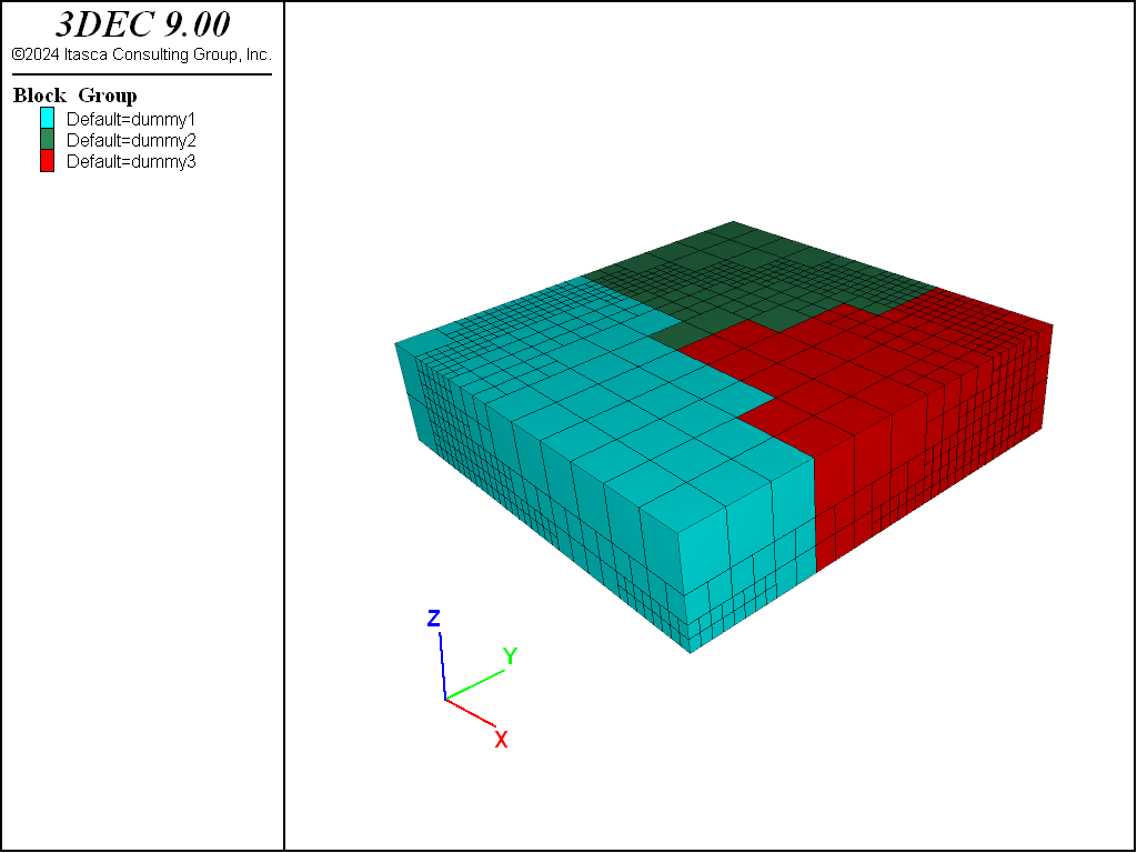
Figure 20: SpaceRanger option 5
Split Large Zones Intersecting Surfaces
Zones that come within 80 m of the surfaces are refined, making sure that no zones less than 40 m are created (see image below).
; Split large zones intersecting surfaces down to no less than 40m
model new
zone create brick size (50,50,50) point 0 (2700,-10500,-1000) ...
		               edge 4000 group 'dummy3'
zone delete range position-z 0 1000000
geometry import 's1.dxf'
zone group 'dummy1' range geometry-space 's1' count 1 direction (0,1,0)
geometry import 's2.dxf'
zone group 'dummy2' ...
           range geometry-space 's2' count 1 direction (1,0,0) group 'dummy3'
geometry import 'Y0.dxf'
geometry import 'Y1.dxf'
geometry import 'Y2.dxf'
zone densify segments 2 edge-limit 50 ...
	range geometry-distance 'Y0' gap 80 extent
zone densify segments 2 edge-limit 50 ...
	range geometry-distance 'Y1' gap 80 extent
zone densify segments 2 edge-limit 50 ...
	range geometry-distance 'Y2' gap 80 extent
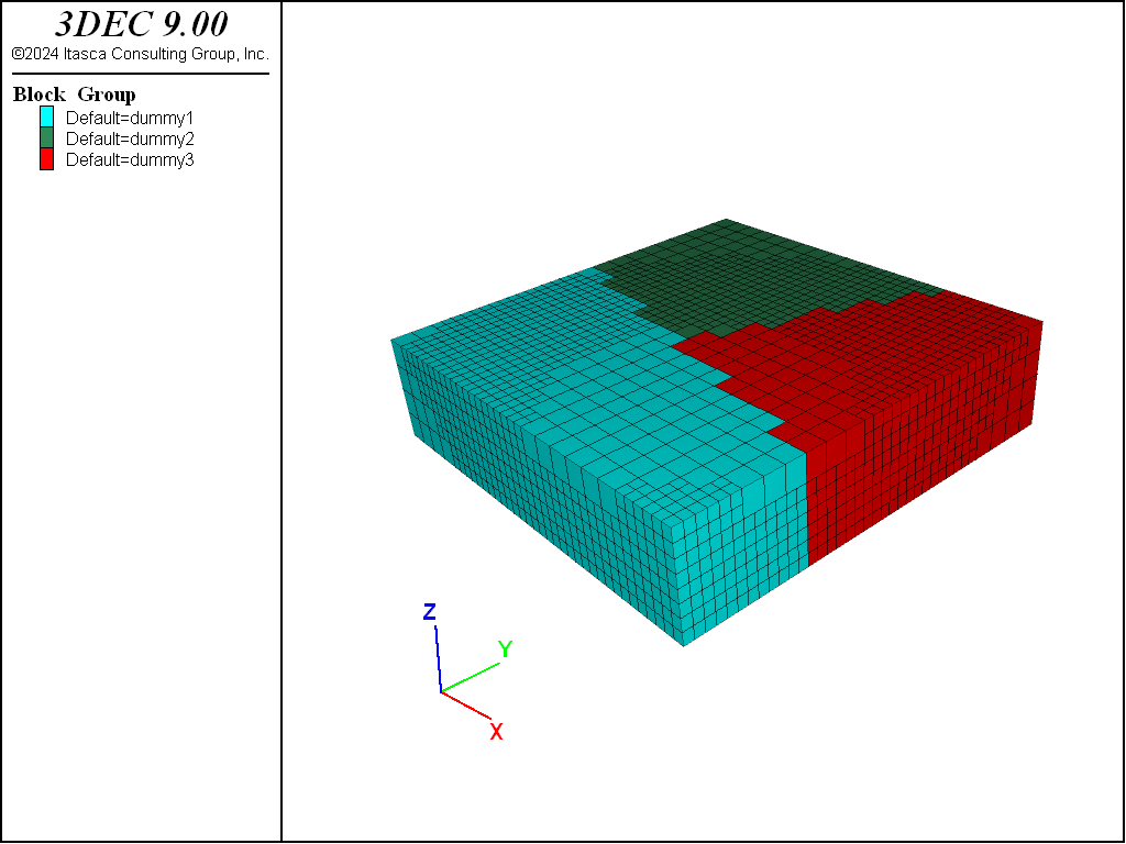
Figure 21: SpaceRanger option 6
| Was this helpful? ... | Itasca Software © 2024, Itasca | Updated: Nov 12, 2025 |
