Examples • Example Applications

Multistage Tunnel Excavation and Support (FLAC2D)

Problem Statement

Note

This project reproduces Example 11 from FLAC 8.1. The project file for this example is available to be viewed/run in FLAC2D.[1] The project’s main data files are shown at the end of this example.

Construction of large railroad, subway, and road tunnels often involves multiple stages of excavation and support, particularly if the tunnels are located at shallow depth and/or in weak ground. A typical example for construction conditions and sequence of a shallow tunnel is illustrated in Figure 1.

In this example, the construction sequence is divided into four major excavation stages:

Stage I: right-side excavation;

Stage II: left-side excavation;

Stage III: top-heading excavation; and

Stage IV: bench excavation.

Each excavation stage is accomplished in three construction steps:

Step a: initial excavation;

Step b: installation of rockbolt support; and

Step c: installation of a shotcrete lining.

The three steps occur at different times during the advancement of the tunnel face. Consequently, the loads acting on the tunnel will be changed at the time the support is installed, as a function of the tunnel advancement.

The stress and displacement fields in the vicinity of a tunnel construction change in the direction of the advancing tunnel face, and this is most rigorously analyzed using a three-dimensional program, such as FLAC3D. However, advancing tunnel problems are often analyzed in two dimensions by neglecting displacements normal to the tunnel cross-section.

An important issue in the design of supports is the amount of change in the tunnel load that takes place due to the tunnel advancement before the support is installed. If no change is assumed to occur, the loads acting on the support will be overpredicted. If complete relaxation at the tunnel periphery is assumed to occur, zero load will develop in the support at the installation step, provided that the relaxation state is at equilibrium. In reality, some relaxation takes place. However, it is difficult to quantify relaxation with a two-dimensional program, because this depends on the distance behind the face at which the support is installed. One way to model the relaxation is to decrease the elastic moduli of the tunnel core, equilibrate, install the support and remove the core. This approach is typical of finite element codes. The main problem then becomes estimating how much to reduce the moduli.

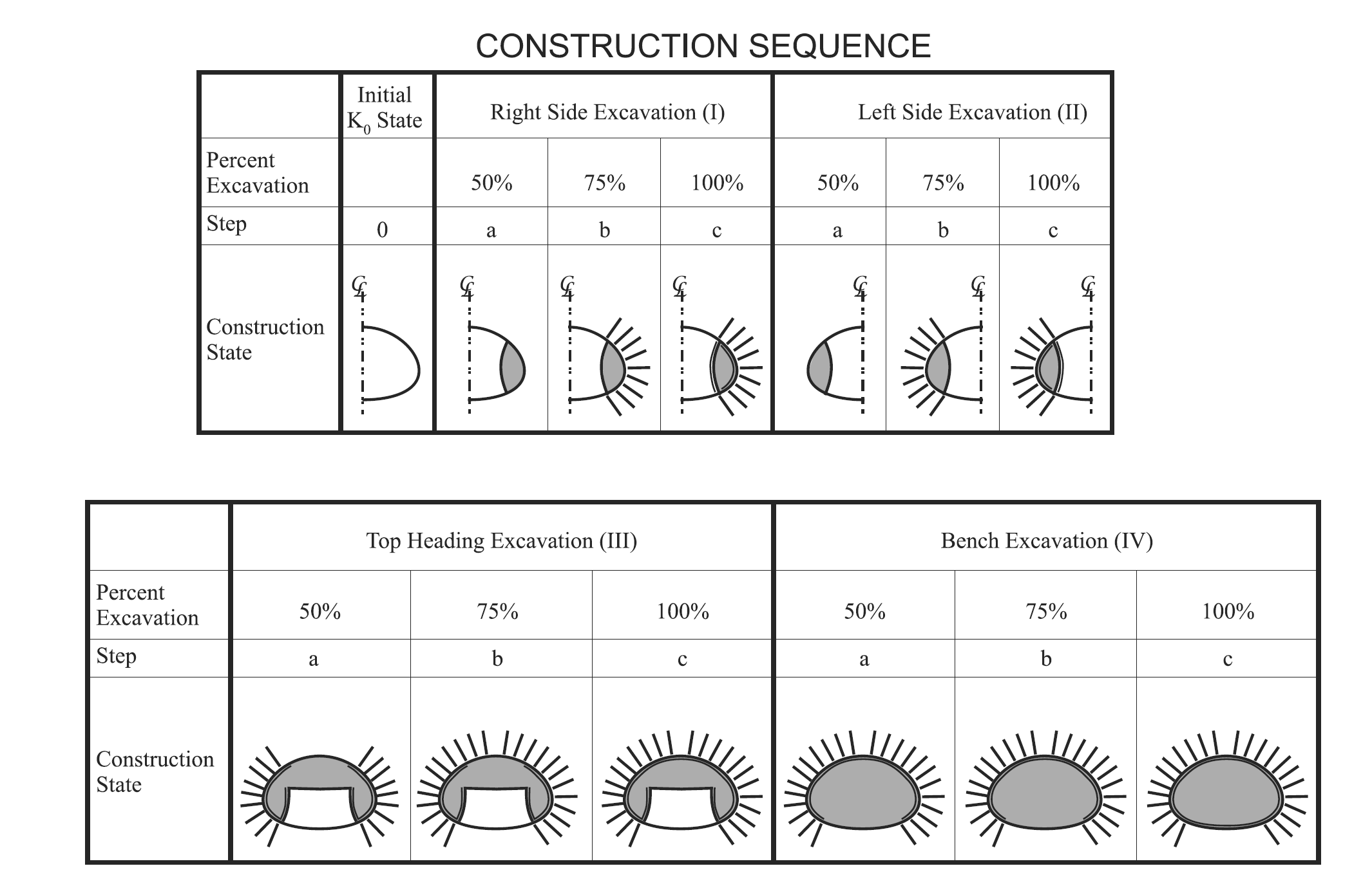
Figure 1: Construction sequence for a multistage tunnel excavation and support.

An alternative approach to model the relaxation is based on the relation of the closure of the unsupported tunnel to the distance to the face. Panet (1979) published such an expression. Tunnel closure can be related to traction forces acting on the tunnel periphery via a ground reaction curve. Thus, the tunnel relaxation as a function of the distance to the face can be specified in terms of tractions defined by a ground reaction curve, and an expression relating closure to distance to the face.

In order to simulate the relaxation, the material modulus of the excavated material is gradually decreased to a value corresponding to a tunnel closure value that is related to a specified distance to the face. The support is then installed at this relaxation state. In this example, the rockbolt support is installed at an excavation stage corresponding to 50% relaxation of the tunnel load, and the shotcrete is installed at a stage corresponding to 75% relaxation, as illustrated in Figure 1.

Modeling Procedure

Model Setup

The tunnel geometry and other construction conditions are shown in Figure 2.

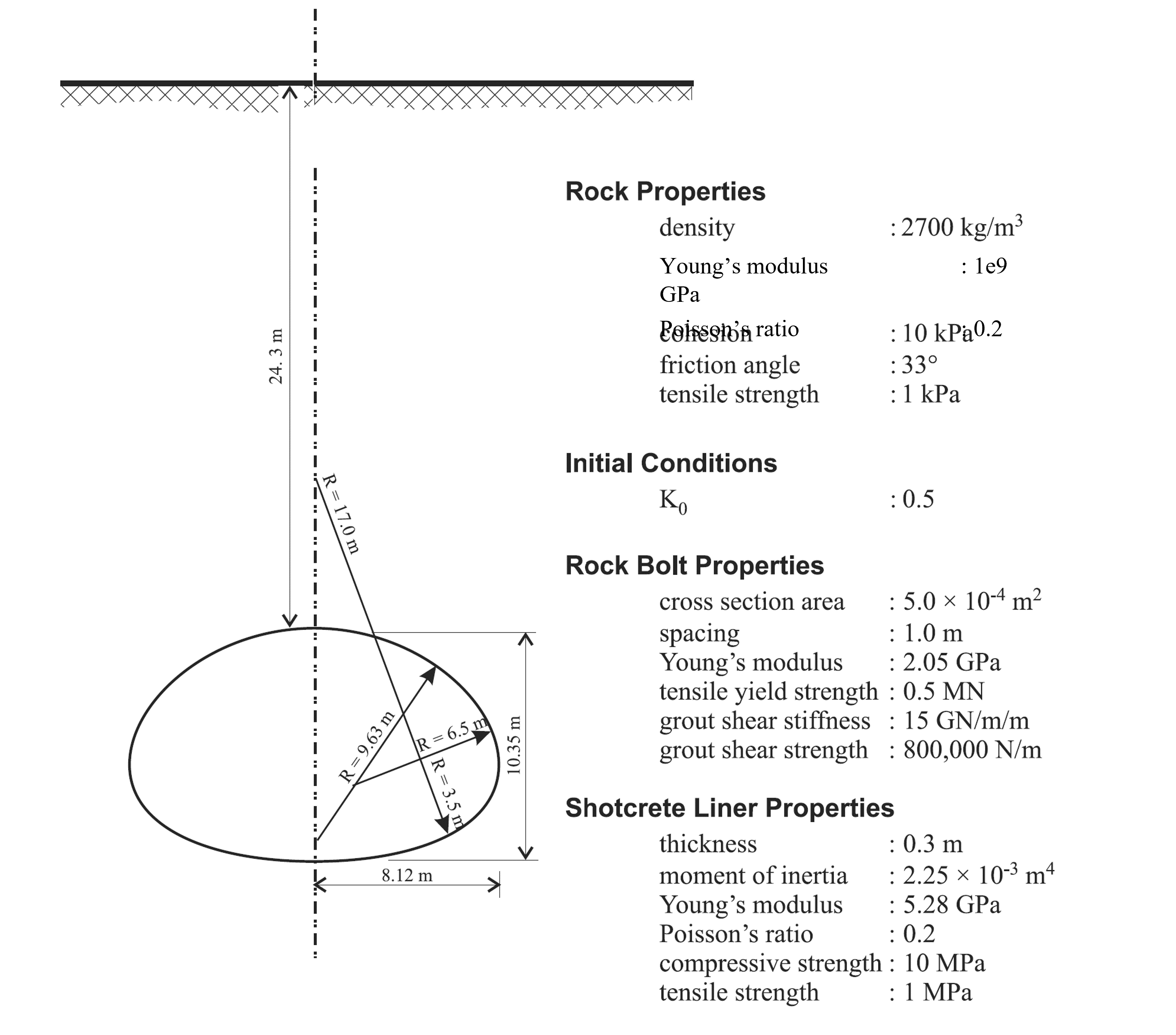
Figure 2: Construction conditions for a multistage tunnel excavation and support.

The tunnel stage boundaries are defined in an imported geometry file, “MultistageTunnel.dxf”. This file can be directly obtained from a CAD drawing or drawn by hand in the Sketch tool. Follow these steps to create the model:

1. Create a new Sketch and import “MultistageTunnel.dxf”. Automatically create points and lines (Figure 3).

2. Mesh the whole model with a zone size of 3.

3. Specify the number of zones for each edge that makes up the tunnel as shown in Figure 4. Tip: Select an edge and then draw a box around the tunnel to select all edges.

4. Mesh all blocks again Figure 5. The mesh may look slightly different since there is some randomness to the unstructured meshing.

5. Specify zone groups as shown in Figure 6. Note that this group assignment could also be done later in the Model Pane.

6. Specify edge groups as shown in Figure 7. Note that this group assignment could also be done later in the Model Pane, but it is easier in Sketch.

7. Generate zones.

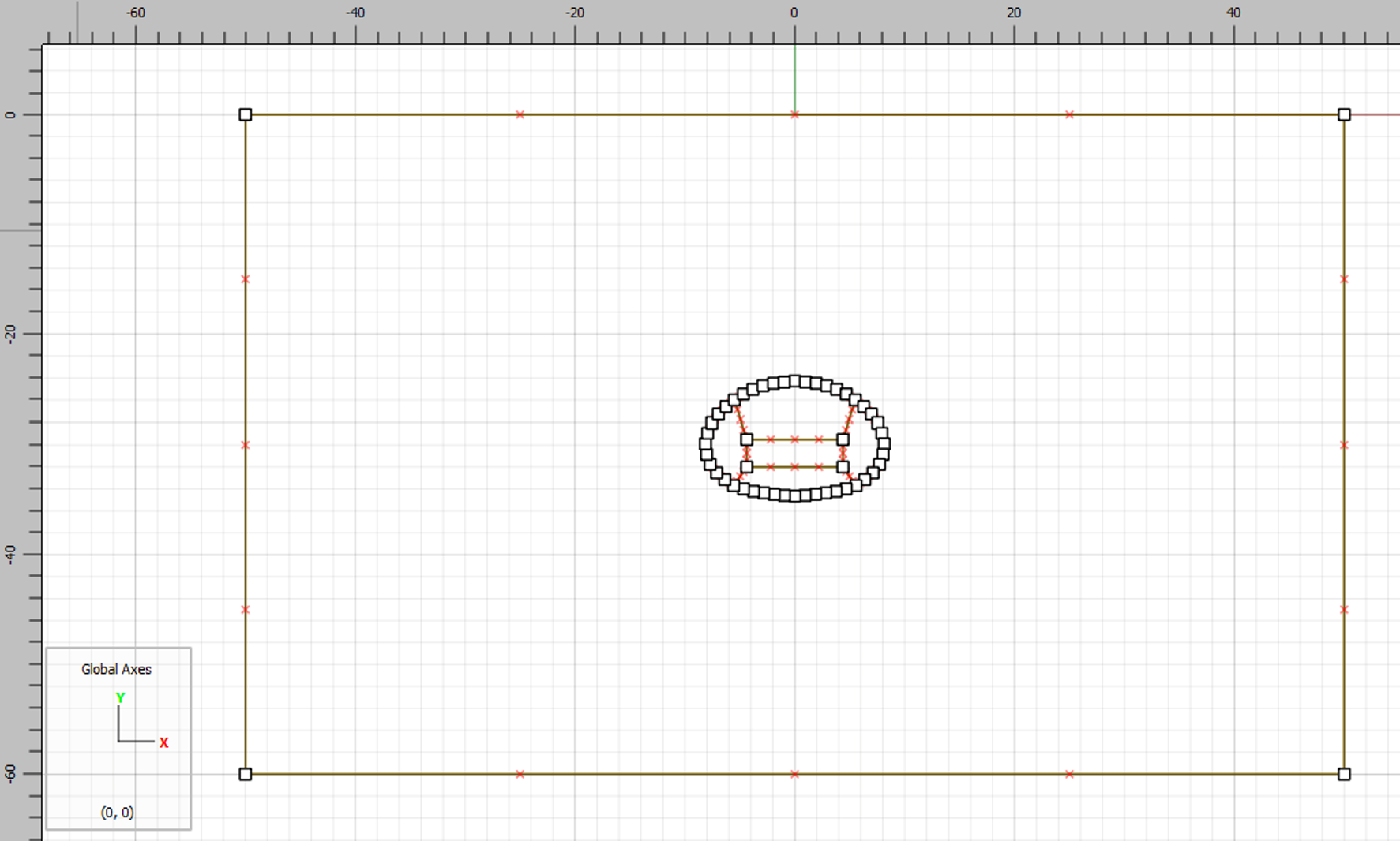
Figure 3: Imported tunnel geometry tuened into nodes and edges.

Figure 4: Number of zones on each edge of the tunnel.

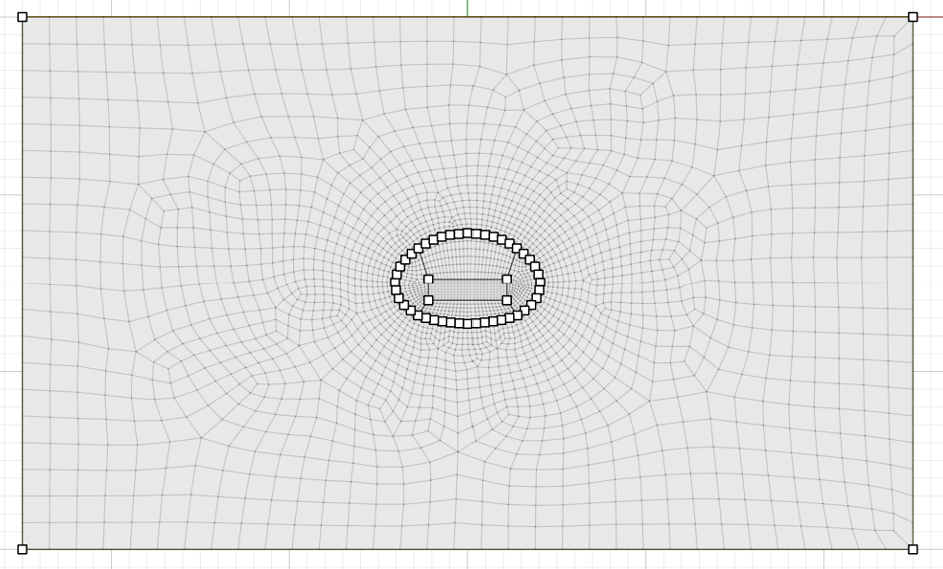
Figure 5: Final mesh.

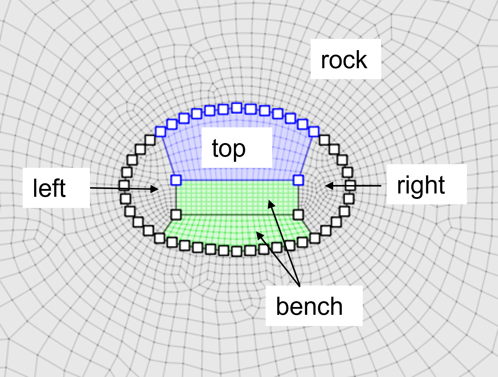
Figure 6: Zone groups assigned in Sketch.

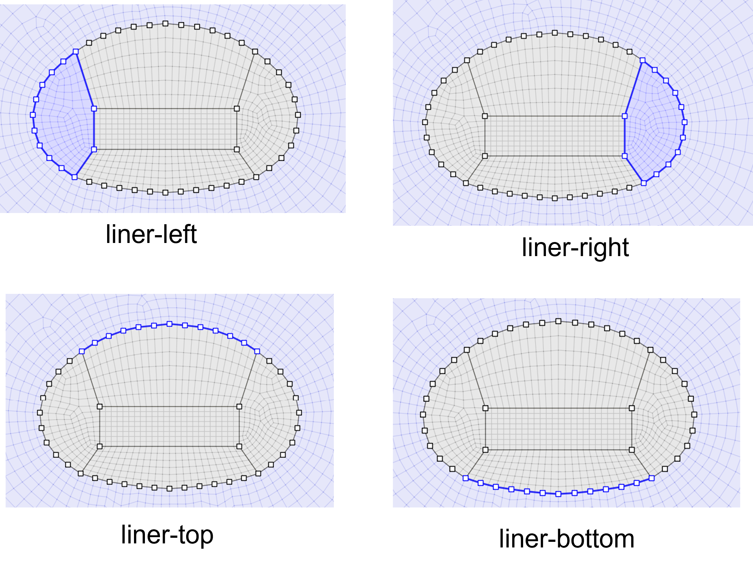
Figure 7: Face groups assigned in Sketch.

In the Model Pane, do the following:

1. Assign Mohr-Coulomb constitutive model to all zones.

2. Set the material properties as shown in Figure 2.

3. Automatically assign face groups, ignoring existing group names.

4. Save the project and the state.

Now, open a data file, restore the previously saved state and set boundary conditions, initial conditions and solve to initial equilibrium as shown in init.dat

Ground Reaction Curve

Before conducting the sequential excavation/support analysis, unsupported tunnel calculations are performed in order to develop ground reaction curves for this model. This procedure is demonstrated for the excavation of the entire tunnel in one stage. Separate ground reaction curves can also be developed for each tunnel segment.

The ground reaction curve is developed by incrementally decreasing the modulus of the material to be excavated while measuring the corresponding tunnel closure. The command zone relax performs this relaxation procedure automatically.

The zone relax command is applied to all zones in the specified range. The rate of modulus decrease is determined by specifying the number of steps over which a linear decrease occurs, a table of decreasing values, or even a FISH function defining the decrease. By default, the modulus is reduced by factors of 0.005 and the model is solved after each reduction. The keyword minimum is used to specify the minimum reduction factor. In this example, the minimum is set to 0.2. If a lower value is specified, the tunnel collapses.

The tunnel closure is monitored as a history. The FISH function closure calculates the vertical closure of the tunnel. The function also calculates the percentage relaxation by dividing the bulk modulus of a zone in the tunnel by its initial bulk modulus. Figure 8 displays the result for load relaxation of the entire tunnel boundary from a relaxation factor of 1.0 to 0.2. This is the ground reaction curve. Note that this is different from the equivalent curve in FLAC 8.1 due to the different method of relaxation. See Appendix to ascertain how to follow the same relaxation procedure as FLAC 8.1 using FISH functions.

The actual curve is not important provided the amount of closure to the distance of the tunnel face from the measurement point can be determined, then reading off the amount of relaxation required to reach the desired state.

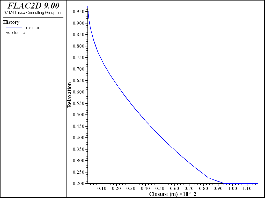
Figure 8: Ground reaction curve: relaxation factor versus vertical closure.

Construction Simulation

The construction steps of the excavation/support analysis follow the same sequence for each excavation stage. First, the modulus of the excavation area is gradually reduced to 50% of its initial value using the zone relax command. This is step a, as shown in Figure 1.

At this state, the cable elements are added, representing the rockbolt support (pile structural elements more accurately model rockbolts, but these require more input parameters and the difference in results in this case is negligible). The locations of the rockbolts for each stage of excavation are defined by a CAD drawing of the rockbolt pattern. This geometry is imported into FLAC2D from DXF files. (The geometry can be imported as a CAD drawing, as shown here, or drawn in the Sketch workspace.) Each rockbolt is composed of five segments, which is sufficient to locate a rockbolt node within every zone along the bolt length.

The modulus of the excavated material is now reduced again to 75% relaxation. This is step b in Figure 1.

At this state, the zones are deleted and the beam elements are added to represent installation of the shotcrete lining. The model is then brought to equilibrium. Note that beams are used instead of liner elements because it is assumed that the shotcrete is perfectly connected to the rock (there is no sliding interface in between). When using beams to represent continuous liners out of the plane, it is necessary to divide the modulus by \(1 - \nu^2\) so the beams are deforming in plane strain rather than plane stress (the default for beams).

Loads that develop in the rockbolts result from tunnel-load relaxation from 50% to zero, and the loads that develop in the shotcrete result from relaxation from 25% to zero.

By applying the relaxation gradually, the effects of transient waves are minimized, and a gradual excavation of the tunnel is simulated. This is demonstrated by Figure 9, which displays vertical stress histories at the springline of the tunnel. The histories show gradual changes in the stresses; if the relaxation loads were applied suddenly (i.e., in one step), sudden changes would be observed in these histories, and a different final state could result. (See Tips and Advice for further discussion on transient effects).

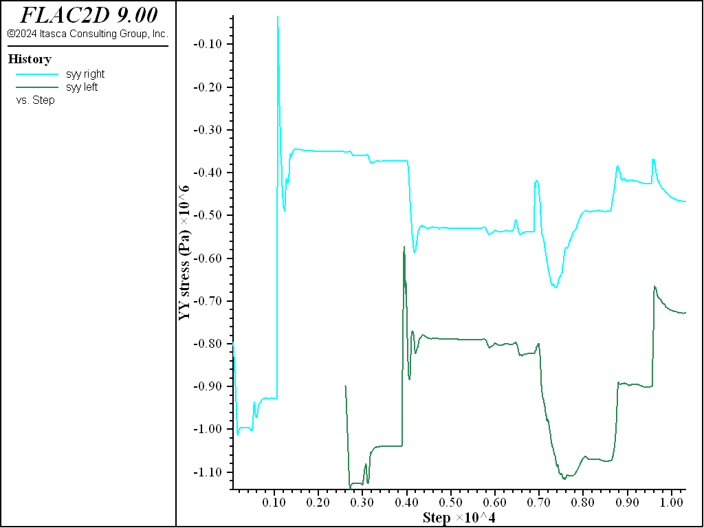
Figure 9: Vertical stress histories at the springline.

Results

Typical results for this analysis are shown in Figure 10 through Figure 13.

The settlement profile of the ground surface at the end of the analysis is shown in Figure 10. The profile is created with the Profile plot item with 50 intervals specified for a line across the top of the model. The contours of displacement in the model are shown in Figure 11. The final axial forces in the rockbolts (cables) are shown in Figure 12, and the liner (beam) axial forces are shown in Figure 13.

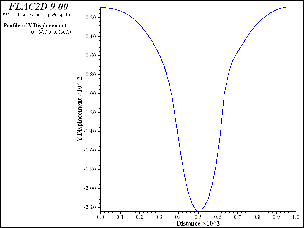
Figure 10: Final settlement profile.

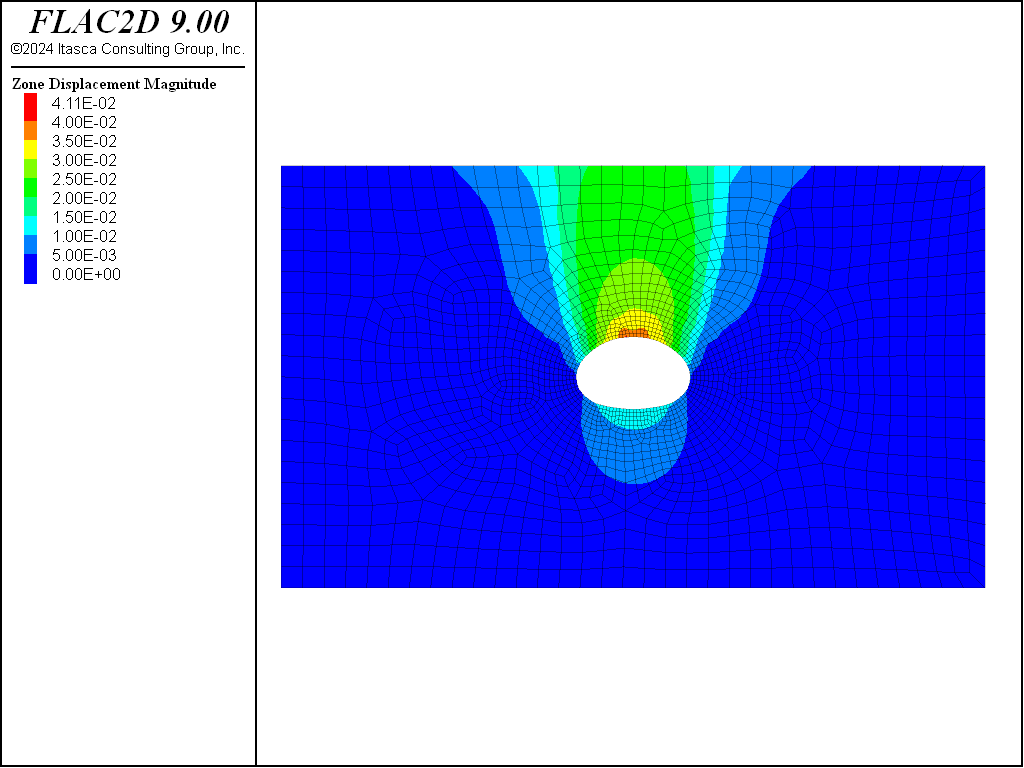
Figure 11: Magnitude of displacement after all excavations.

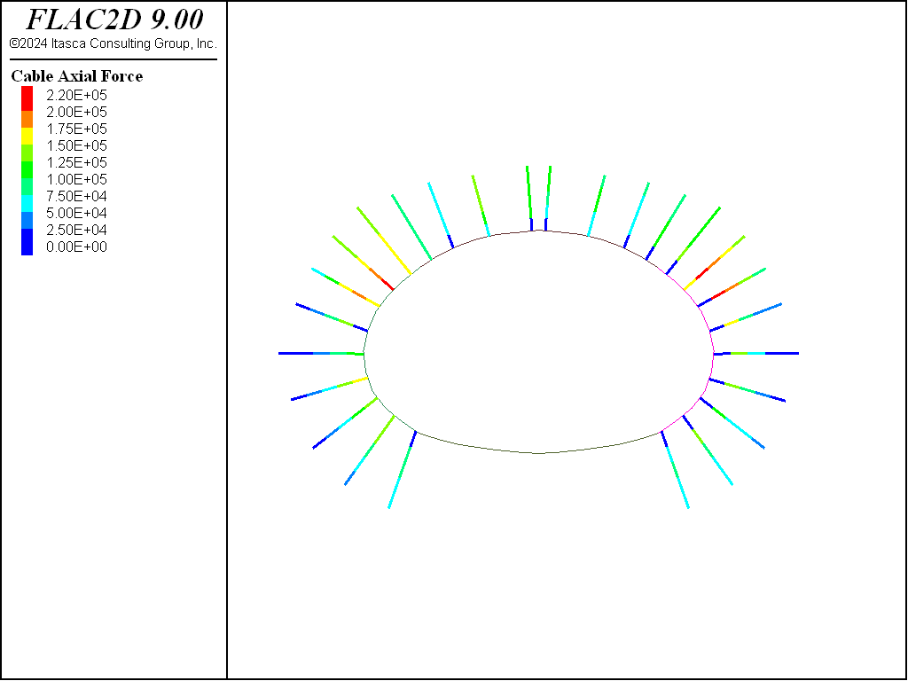
Figure 12: Final axial forces in rockbolts (cables).

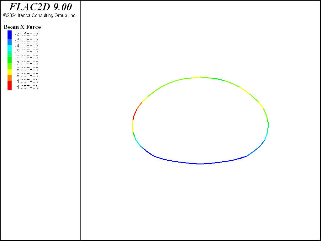
Figure 13: Final axial forces in liners (beams).

Reference

Panet, M. “Time-Dependent Deformations in Underground Works,” in Proceedings of the 4th ISRM Congress (Montreux), Vol. 3, pp. 279-289. Rotterdam: A. A. Balkema and the Swiss Society for Soil and Rock Mechanics (1979).

Data File

init.dat

;==========================================

model restore 'MST-grid'

model gravity 9.81
zone initialize-stresses ratio 0.5

zone face apply velocity-x 0 range group "East" or "West"
zone face apply velocity 0 0 range group "Bottom"

model large-strain off
model solve elastic
;
model save 'MST-initial'

Right-side.dat

model restore 'MST-initial'
;
; relax to 50%
zone relax excavate minimum 0.5 range group 'right'
zone history name 'syy right' stress-yy position 8.4 -30
model solve

; add rock bolts
geometry import 'rockbolts-right.dxf'
structure cable import from-geometry 'rockbolts-right' segments 5
structure cable property cross-sectional-area=5e-4 young=205e9 ...
                      yield-tension=5e5 grout-stiffness=1.5e10 grout-cohesion=8e5

; note, this is 50% of 50%, to get to 25% relax
zone relax excavate minimum 0.5 range group 'right'
model solve

; delete zones
zone delete range group 'right'
;
; add liner - use beams so we don't have to specify contact properties
; but be careful to divide E by 1-v^2
structure beam create by-zone-face range group 'liner-right'
structure beam property young=[5.5e9/(1.0-0.2^2)] poisson=0.20
structure beam property cross-sectional-area=0.1 moi=8.333e-5 
;
model solve
model save 'MST-right'

Left-side.dat

model restore 'MST-right'
;
; relax to 50%
zone relax excavate minimum 0.5 range group 'left'
zone history name 'syy left' stress-yy position -8.4 -30
model solve

; add rock bolts
geometry import 'rockbolts-left.dxf'
structure cable import from-geometry 'rockbolts-left' segments 5
structure cable property cross-sectional-area=5e-4 young=205e9 ...
                      yield-tension=5e5 grout-stiffness=1.5e10 grout-cohesion=8e5

; note, this is 50% of 50%, to get to 25% relax
zone relax excavate minimum 0.5 range group 'left'
model solve

; delete zones
zone delete range group 'left'
;
; add liner 
structure beam create by-zone-face range group 'liner-left'
structure beam property young=[5.5e9/(1.0-0.2^2)] poisson=0.20
structure beam property cross-sectional-area=0.1 moi=8.333e-5 
;
model solve
model save 'MST-left'

top.dat

model restore 'MST-left'
;
; relax to 50%
zone relax excavate minimum 0.5 range group 'top'
model solve

; add rock bolts
geometry import 'rockbolts-top.dxf'
structure cable import from-geometry 'rockbolts-top' segments 5
structure cable property cross-sectional-area=5e-4 young=205e9 ...
                      yield-tension=5e5 grout-stiffness=1.5e10 grout-cohesion=8e5

; note, this is 50% of 50%, to get to 25% relax
zone relax excavate minimum 0.5 range group 'top'
model solve

; delete zones
zone delete range group 'top'

; manually delete beams no longer connected to zones!
structure beam delete range position-x -5.5 5.5 position-y -29.5 -26
;
; add liner 
structure beam create by-zone-face range group 'liner-top'
structure beam property young=[5.5e9/(1.0-0.2^2)] poisson=0.20
structure beam property cross-sectional-area=0.1 moi=8.333e-5 
;
model solve
model save 'MST-top'

bench.dat

model restore 'MST-top'
;
; no bolts.  Relax to 25%
zone relax excavate minimum 0.25 range group 'bench'
model solve

; delete zones
zone delete range group 'bench'

; manually delete liner
structure beam delete range position-x -5.5 5.5 position-y -33.7 -29.5
;
; add liner 
structure beam create by-zone-face range group 'liner-bottom'
structure beam property young=[5.5e9/(1.0-0.2^2)] poisson=0.20
structure beam property cross-sectional-area=0.1 moi=8.333e-5 
;
model solve
model save 'MST-bottom'

ground-reaction.dat

model restore 'MST-initial'

; get variables required to generagte ground reaction curve
fish define reaction_ini
  topgp = gp.near(0,-24.28)
  bottomgp = gp.near(0,-34.65)
  zone_tunnel = zone.near(0,-30)
  zone_bulk_ini = zone.prop(zone_tunnel,'bulk')
end
[reaction_ini]

fish define closure
   closure = gp.dis.y(bottomgp) - gp.dis.y(topgp)
   relax_pc = zone.prop(zone_tunnel,'bulk')/zone_bulk_ini
end

fish history name 'closure' closure
fish history name 'relax_pc' relax_pc

zone relax excavate minimum 0.2 range group 'top' or 'bench' or 'left' or 'right'

model solve

Appendix

The gradual excavation of the tunnel can also be preformed by deleting the zones in the tunnel and applying forces to the tunnel surface equal and opposite to the unbalanced forces, and then gradually reducing them. This methodology is shown in the data file below (ground-reaction-2.fis). If this method is used, then the ground reaction curve is essentially the same as that shown in Example 11 of the FLAC 8.1 manual.

model restore 'MST-initial'

; set all tunnel sections to be the same group
zone group 'tunnel' slot 'grc' range group 'Top' or 'Left' or 'Right' or 'Bench'

; identify gridpoints at intersection of tunnel and rock
zone gridpoint group 'tunnel_bound' range group 'tunnel' group 'rock'

; create list of gridpoints on the boundary
; see FISH splitting in the documentation to understand this syntax
[gp_bound = gp.list(gp.isgroup(::gp.list,'tunnel_bound'))]

; delete zones
zone delete range group 'tunnel'

; cycle 1 to set up unbalanced forces
model cycle 1

; store unbalanced forces (opposite)
fish define store_forces
  loop foreach gp gp_bound
    gp.extra(gp) = -gp.force.unbal(gp)
  end_loop
end
[store_forces]

; functions to get closure
[topgp = gp.near(0,-24.28)]
[bottomgp = gp.near(0,-34.65)]
fish define closure
   closure = gp.dis.y(bottomgp) - gp.dis.y(topgp)
end

; now apply equal and opposite forces and gradually reduce them
fish define reduce
  cycle0 = mech.cycle
  grc = table.get('grc')
  
  ; do 8 equal increments - only reducing to a factor of 0.2
  loop i (1,9)
    reduction_factor = 1.0 - (i-1)/10.0 
    loop foreach gp gp_bound
      gp.force.load(gp) = gp.extra(gp)*reduction_factor
    end_loop
    command
      model solve
    end_command
    
    ; dump results to table
    table.value(grc,i) = vector(closure,reduction_factor)
  end_loop
end
[reduce]

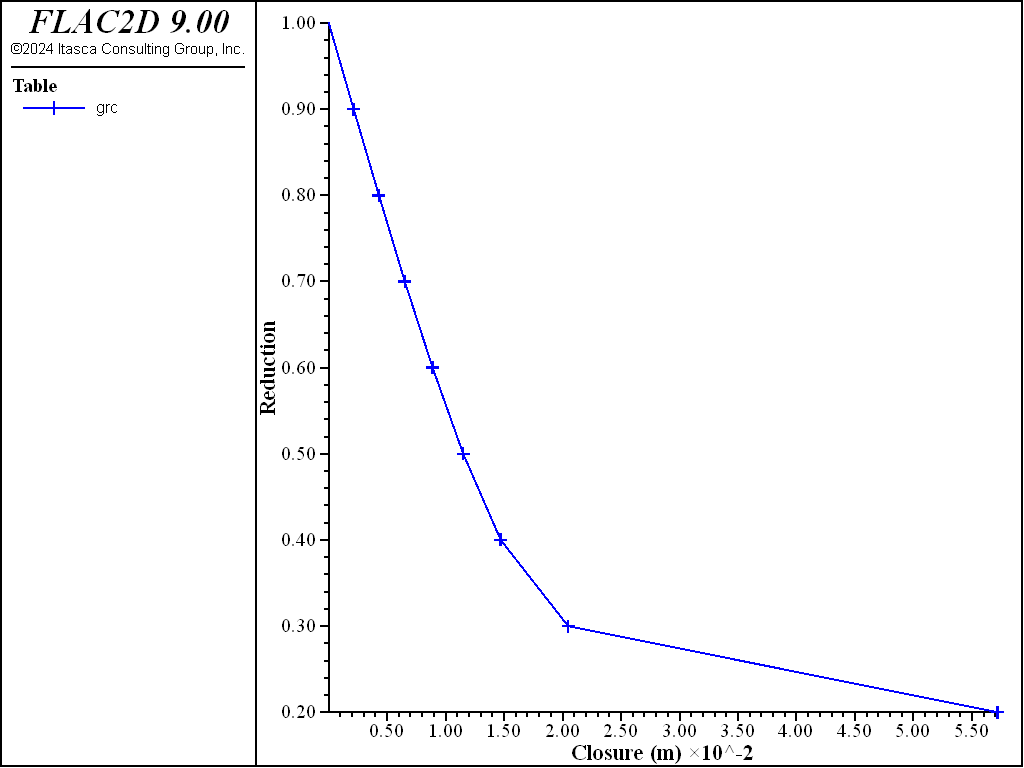
Figure 14: Ground reaction curve obtained by reducing applied forces on the tunnel boundary.

Endnotes

[1]

To view this project in FLAC2D, use the program menu.

Help ▼ Examples…

  ⮡   FLAC
   ⮡   Example Applications
    ⮡   FromFLAC
     ⮡   11MultiStageTunnel
     ⮡   MST.prj