Smooth Circular Footing on an Associated Mohr-Coulomb Material (FLAC2D)
Problem Statement
Note
The project file for this example is available to be viewed/run in FLAC2D.[1] The project’s main data file is shown at the end of this example.
The prediction of collapse loads under steady plastic flow conditions can be difficult for a numerical model to simulate accurately (Sloan and Randolph 1982). A simple example of a problem involving steady-flow is the determination of the bearing capacity of a footing on an elastic-plastic soil. The bearing capacity is dependent on the steady plastic flow beneath the footing, thereby providing a measure of the ability of FLAC2D to model this condition.
The bearing capacity of a smooth circular footing on a Mohr-Coulomb medium is determined numerically in this example. The footing with radius \(a\) is located on an associated material with the following properties:
shear modulus (\(G\)) |
0.1 GPa |
bulk modulus (\(K\)) |
0.2 GPa |
cohesion (\(c\)) |
0.1 MPa |
friction angle (\(\phi\)) |
20° |
dilation angle (\(\psi\)) |
20° |
Semi-Analytical Solution
Cox et al. (1961) have numerically solved the slip-line equations for this axisymmetric-footing problem. The semi-analytical value of the average pressure over the footing at failure for a friction angle of 20° is found to be
in which \(q\) is the bearing capacity and \(c\) is the cohesion of the material. The corresponding slip-line net, as referenced in Chen (1975), is sketched in Figure 1.

Figure 1: Cox slip-line net for a smooth circular footing at \(\phi\) = 20°.
FLAC2D Model
The problem is solved in FLAC2D using axisymmetric mode (model configure axisymmetry). With this, the circular footing is represented in the model by a linear segment of length \(a\) = 3 m. Boundary conditions applied to the model and overal dimensions of the model are provided in Figure 2 and Figure 3 below.
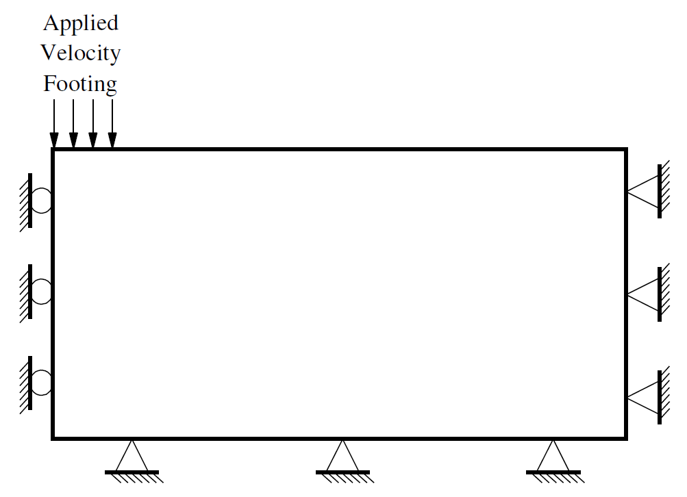
Figure 2: Boundary conditions for FLAC2D axisymmetric model.
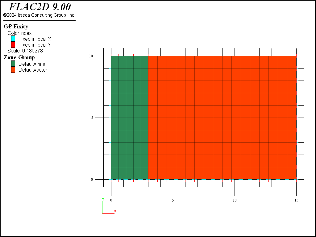
Figure 3: Axisymmetric model domain and grid.
The domain is discretized into a regular pattern of 210 zones, as represented in Figure 3. The effective radius, \(R\), representing the footing, extends for five zones in the radial \(x\)-direction—over which the velocity is applied—plus half the distance to the gridpoints adjacent to the last gridpoints with applied velocity. As a velocity is applied to gridpoints to simulate a footing load, the bearing area is found by assuming that the velocity varies linearly from the value at the last applied gridpoint to zero at the next gridpoint.
The velocity magnitude is set to 2.5 × 10⁻⁵ m/step and it is applied at the footing nodes for a total of 10000 timesteps.
The FISH function load contained in the file footing-load.dat computes the numerical value of the normalized average footing pressure, \(p/c\).
Results and Discussion
The load-displacement curve corresponding to the numerical simulation is presented in Figure 4, in which load is the normalized average footing pressure, \(p/c\), anaval is the analytical value of the normalized bearing capacity, \(q/c\), and disp is the normalized vertical displacement, \(u_y/a\).
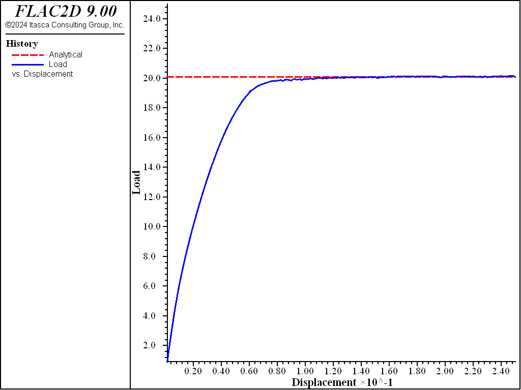
Figure 4: Load-displacement curve.
In order to calculate normalized average footing pressure, \(p/c\), the following expression is used
where: |
\(f_{i}^{y}\) |
= |
reaction force in the \(y\)-direction at footing gridpoint \(i\); |
\(r_i\) |
= |
associated radius at gridpoint \(i\); |
|
\(R\) |
= |
effective radius of the footing (as defined earlier); and |
|
\(\Sigma\) |
= |
summation over all gridpoints with applied velocity |
For gridpoints not on the axis of symmetry, the associated radius \(r_i\) is the radial distance to each gridpoint that has an applied velocity. At the left-most gridpoint, the associated radius is 0.25 times the radius to the next gridpoint with applied velocity.
Velocity contours and velocity vectors at the end of the run are presented in Figure 5, showing good agreement with the mechanism in Figure 1.
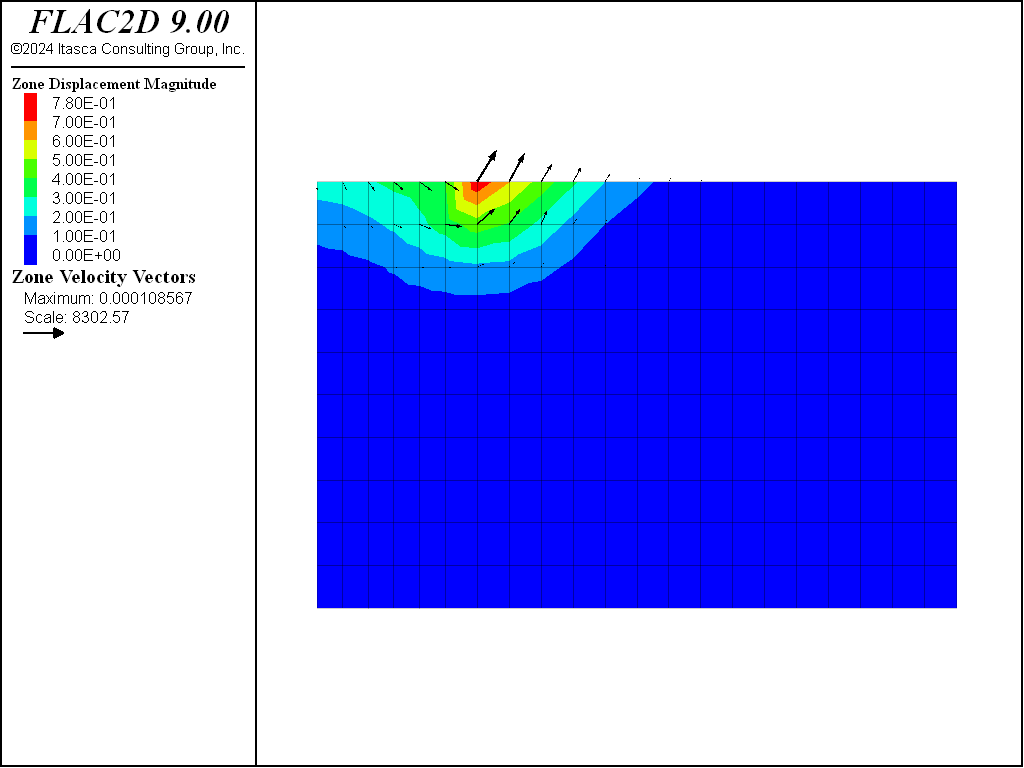
Figure 5: Velocity field at collapse load.
References
Chen, W.-F. “Bearing Capacity of Square, Rectangular and Circular Footings,” in Limit Analysis and Soil Plasticity, Developments in Geotechnical Engineering 7, Ch. 7, pp. 295-340, New York: Elsevier Scientific Publishing Co. (1975).
Cox, A. D., G. Eason and H. G. Hopkins. “Axially Symmetric Plastic Deformation in Soils,” Phys. Trans. Royal Soc. London, Series A, 254(1036), 1-45 (1961).
Sloan, S.W., and M. F. Randolph. “Numerical Prediction of Collapse Loads Using Finite Element Methods,” Int. J. Num. & Analy. Methods in Geomech., 6, 47-76 (1982).
Data File
CircularFooting.dat
;---------------------------------------------------------------------
; circular smooth footing on Mohr-Coulomb material (Cox problem)
;   -associated plastic flow-
;---------------------------------------------------------------------
model new
model large-strain off
model configure axisymmetry
; Create zones
zone create2d quadrilateral point 0 (0,0) point 1 (3,0)  point 2 (0,10) ...
              size 5 10 group "inner"
zone create2d quadrilateral point 0 (3,0) point 1 (15,0) point 2 (3,10) ...
              size 16 10 group "outer"

; Assign constitutive model and properties
zone cmodel assign mohr-coulomb
zone property bulk 2.e8 shear 1.e8 cohesion 1.e5
zone property friction 20. dilation 20. tension 1.e10
; Name surfaces
zone face skin
zone face group 'slab' range group 'inner' group 'Top'
; Boundary Conditions
zone face apply velocity-normal -2.5e-5 range group 'slab'
zone face apply velocity (0,0) range group 'Bottom'
zone face apply velocity (0,0) range group 'East'
; call FISH function that calculates footing load
program call 'footing-load'
; Take some histories
history interval 50
fish history [load]
fish history [anaval]
fish history [disp]
model history mechanical ratio-local
; Cycle till stable velocity field
model cycle 10000
; Save the model
model save 'cox'

fish list [load]
fish list [anaval]
fish list [err]
Endnote
| Was this helpful? ... | Itasca Software © 2024, Itasca | Updated: Nov 12, 2025 |
