Steady-State Fluid Flow with a Free Surface (FLAC2D)

Problem Statement

Note

The project file for this example is available to be viewed/run in FLAC2D.[1] The main data files used are shown at the end of this example. The remaining data files can be found in the project.

This numerical simulation analyzes the steady-state seepage flow through a homogeneous embankment with vertical slopes exposed to different water levels and resting on an impermeable base. The total discharge, Q, and the length of seepage face, s, are compared to the exact solutions. The problem tests FLAC2D’s formulation for unconfined groundwater flow. Figure 1 shows the geometry and boundary conditions of the problem.

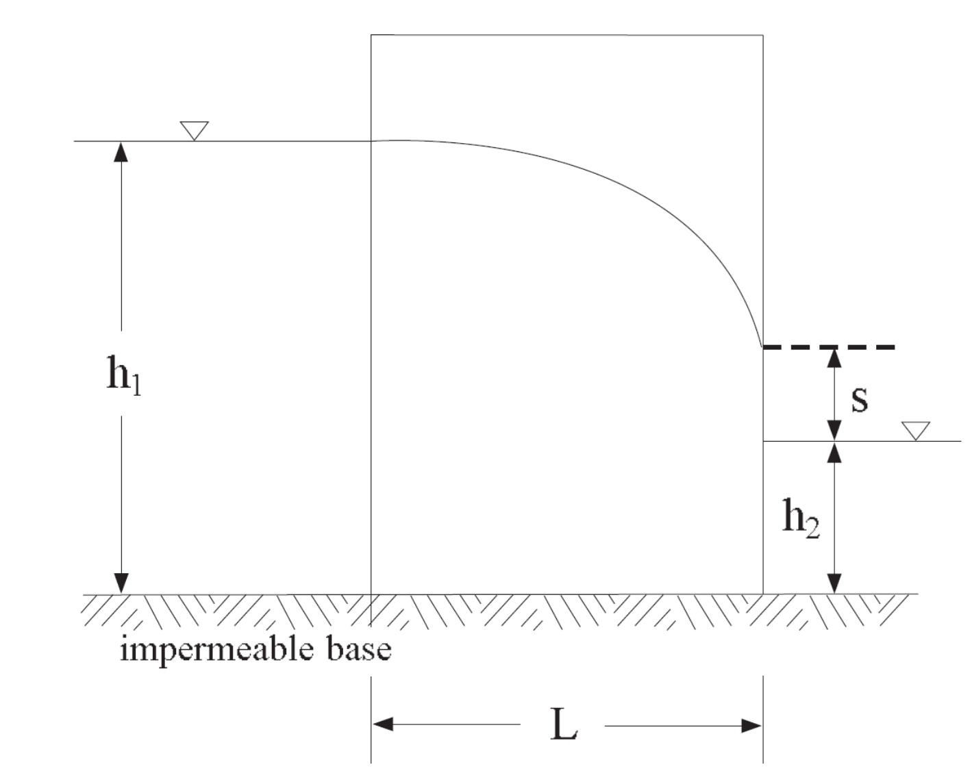
Figure 1: Problem geometry and boundary conditions.

The dimension and elevations are:

\(L\)	= 9 m
\(h_1\)	= 6 m
\(h_2\)	= 1.2 m

The following material properties are used.

permeability (k)	10−10 (m/sec)/(Pa/m)
porosity (n)	0.3
water density (ρw)	1000 kg/m3
water bulk modulus (Kw)	1000 Pa
soil dry density (ρ)	2000 kg/m3
gravity (g)	10 m/sec:sup:\(2\)

Analytic Solution

Dupuit’s formula (see, for example, Davis and DeWiest 1966, p. 186) gives the exact solution for the total flow rate (per unit model thickness) as

\[Q = k \ \rho_w \ g \cdot \frac{h^2_1 - h^2_2}{2L}\]

For this particular case, the value for \(Q\) is 1.92 × 10−6 m³/s. The length, s, of the seepage face as a function of the characteristic dimensions of the section was obtained by Polubarinova-Kochina and is given in Figure 2 (see, e.g., Harr 1991, pp. 206-207). For this particular problem, \(h_2/h_1 = 0.2\), \(L/h_1 = 1.5\), and the value of \(s/h_1\) is evaluated from the graphs at 0.1, which gives an elevation \(s\) = 0.6 m.

FLAC2D Model

Two cases have been studied, corresponding to two different initial conditions:

CASE 1: The embankment is initially dry (saturation = 0), and the sides are suddenly exposed to the water.

CASE 2: The water level at both sides is initially the same (\(h_1\) = \(h_2\) = 6 m), followed by a sudden drawdown at the right side (\(h_2\) = 1.2 m).

The grid and boundary conditions are the same for both cases . The only difference is the initial pore-pressure distribution. In Case 1, saturation and pore pressure are zero inside the mesh; in Case 2, saturation is 1 for all gridpoints, and the pore pressure inside the mesh follows a gravitational gradient.

The material properties are assigned as described above. Because only the steady-state fluid flow solution is of interest in this problem, the mechanical behavior of the soil and its interaction with the groundwater flow are not addressed. The absolute values of soil density, homogeneous permeability and porosity are not relevant to the final solution, and the water bulk modulus is given a small value, compatible with free surface numerical stability, to speed up the calculation to steady state.

Figure 2: Seepage face solution after Polubarinova-Kochina

Results and Discussion

The flow simulation for the two cases is carried out using the MODEL SOLVE command. The evolution toward steady state is monitored using the FISH function flow, which calculates inflow and outflow at the left model boundary and right model boundary, respectively. Inflow is positive if water flows into the model, while outflow is positive if water flows out; at steady state, the free surface is a streamline, and inflow is equal to outflow.

The evolutions of the inflow and outflow rates are plotted and compared to the analytical steady-state solution (shown as a solid line) in Figure 3 and Figure 4. The difference in the flow patterns leading to steady-flow is seen by comparing Figure 5 and Figure 6, which show the flow vectors after 500 steps for Case 1 and 2, respectively.

In both cases, the final flow pattern is similar (see Figure 7 and Figure 8). The calculated length of seepage extends in those figures from the tail water elevation up to the point on the downstream embankment slope where the magnitude of the flow vector becomes zero. As may be seen, the numerical seepage length compares well with the sketched analytical solution.

Figure 3: Flow rate evolution (Case 1).

Figure 4: Flow rate evolution (Case 2).

Figure 5: Flow vectors after 500 steps (Case 1).

Figure 6: Flow vectors after 500 steps (Case 2).

Figure 7: Steady-state flow vectors and seepage face solution (Case 1).

Figure 8: Steady-state flow vectors and seepage face solution (Case 2).

References

Davis, S. N., and R. J. DeWiest. Hydrogeology. J. Wiley (1966).

Harr, M. E. Groundwater and Seepage. Dover (1991).

Data Files

FreeSurfaceInitialDry.dat

;-----------------------------------------------------------
;    Steady-State Fluid Flow with a Free Surface
;-----------------------------------------------------------
model new
model large-strain off
fish automatic-create off
model title "Steady-State Fluid Flow with a Free Surface   "
model config fluid
program call 'fishfunctions.dat'
[setup]
; --- model geometry ---
zone create quadrilateral size 30 20 p 1=([bl],0.0) p 2=(0.0,[h1]) p 3=([bl],[h1])
zone face skin
zone cmodel assign elastic
zone property density 2000.0
; --- fluid properties ---
zone fluid cmodel assign isotropic
zone fluid property permeability [ck] porosity 0.3
zone gridpoint initialize fluid-modulus 1e3
zone initialize fluid-density [rw]
; --- initial conditions ---
zone gridpoint initialize saturation 0.0
; --- boundary conditions ---
zone face apply pore-pressure 6e4 grad 0 -1.0e4 range group 'West'
zone face apply pore-pressure 1.2e4 gradient 0 -1.0e4 ...
                range group 'East' position-y 0.0 1.2
zone gridpoint initialize saturation 1.0 range group 'West'
zone gridpoint initialize saturation 1.0 range group 'East' position-y 0.0 1.2
; --- settings ---
model mechanical active off fluid active on
model gravity  0 -10
; --- Fish functions ---
[global pnt1= list(gp.list)(gp.isgroup(::gp.list,"West"))]
[global pnt2 =list(gp.list)(gp.isgroup(::gp.list,"East"))]
fish define flow
  global inflow
  global outflow
  local sum1=0.0
  local sum2=0.0
  sum1 =list.sum(gp.flow(::pnt1))
  sum2 =-1.0*list.sum(gp.flow(::pnt2))
  inflow=sum1
  outflow =sum2
  flow=qt
end


; --- histories ---
history interval 50
zone history pore-pressure position (4.3,0.16)

fish history flow
fish history inflow
fish history outflow

; --- step ---
model step 500
model save 'h2aa'
model solve fluid ratio-flow  1e-6
model save 'h2a'

FreeSurfaceInitialSaturated.dat

;-----------------------------------------------------------
;    Steady-State Fluid Flow with a Free Surface
;-----------------------------------------------------------
model new
model large-strain off
fish automatic-create off
model title "Steady-State Fluid Flow with a Free Surface   "
model config fluid
program call 'fishfunctions.dat'
[setup]
; --- model geometry ---
zone create quadrilateral size 30 20 p 1=([bl],0.0) p 2=(0.0,[h1]) p 3=([bl],[h1])
zone face skin
zone cmodel assign elastic
zone property density 2000.0
; --- fluid properties ---
zone fluid cmodel assign isotropic
zone fluid property permeability [ck] porosity 0.3
zone gridpoint initialize fluid-modulus 1e3
zone initialize fluid-density [rw]
; --- initial conditions ---
zone gridpoint initialize saturation 1.0
zone gridpoint initialize fluid-tension 0.0
; --- boundary conditions ---
zone gridpoint initialize pore-pressure 6e4 grad 0 -1.0e4
zone gridpoint fix pore-pressure range group 'West'
zone face apply pore-pressure 1.2e4 gradient 0 -1.0e4 ...
                range group 'East' position-y 0.0 1.2
zone face apply pore-pressure 0.0 range group 'East' position-y 1.5 6.0
; --- settings ---
model mechanical active off fluid active on
model gravity  0 -10
; --- Fish functions ---
[global pnt1= list(gp.list)(gp.isgroup(::gp.list,"West"))]
[global pnt2 =list(gp.list)(gp.isgroup(::gp.list,"East"))]
fish define flow
  global inflow
  global outflow
  local sum1=0.0
  local sum2=0.0
  sum1 =list.sum(gp.flow(::pnt1))
  sum2 =-1.0*list.sum(gp.flow(::pnt2))
  inflow=sum1
  outflow =sum2
  flow=qt
end

; --- histories ---
history interval 50
zone history pore-pressure position (4.3,0.16)

fish history flow
fish history inflow
fish history outflow

; --- step ---
model step 500
model save 'h2bb'
model solve fluid ratio-flow  1e-6
model save 'h2b'

fishfunctions.dat

fish define setup
   global h1 = 6.
   global h2 = 1.2
   global bl = 9.
   global ck = 1e-10
   global rw = 1e3
   global gr = 10.
   global qt = ck*rw*gr*(h1*h1 - h2*h2)/(2.0*bl)
end

[1]

To view this project in FLAC2D, use the program menu.

Help ▼ Examples…

  ⮡   FLAC
   ⮡   VerificationProblems
    ⮡   SteadyFlowWithFreeSurface
     ⮡   SteadyFlowWithFreeSurface.prj