Columnar-Basalt Model: Unconfined Compression Test
Note
To view this project in FLAC3D, use the menu command . The project’s main data files are shown at the end of this example.
Unconfined visco-elastic element tests under constant vertical pressure P are conducted with the COMBA model and one active ubiquitous joint. The element is represented in Figure 1. The ubiquitous joint makes an angle with the horizontal plane. The local axes are indicated with a prime.
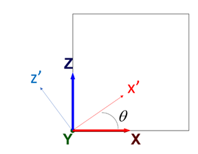
Figure 1: Element and ubiquitous joint representation.
Analytical Solution
The local vertical stress, shear stress, and Coulomb shear stresses are as follows.
where \(\sigma_{zz} = -P\), \(c\) is the joint cohesion, and \(\phi\) is joint friction. By definition of the creep rate:
After using the expressions (1) to express (2)) in terms of \(\sigma_{zz}\) and integrating with time, we obtain:
Finally, the global strains are obtained using the following expressions:
Numerical Solution
An example data for the simulation is listed in the data file below. The creep properties are: \(A\) = 0.002, \(n\) = 4, and \(s_{lim}\) = 0. The joint cohesion is 1, and friction is zero. The displacements obtained at the end of the simulation are shown in Figure 2 to Figure 7 for different values of the ubiquitous joint angle (counted positive counter-clockwise from the horizontal plane). A comparison between numerical prediction (blue line) and analytical value (red symbol) of vertical displacement is shown versus creep time on the same plot.
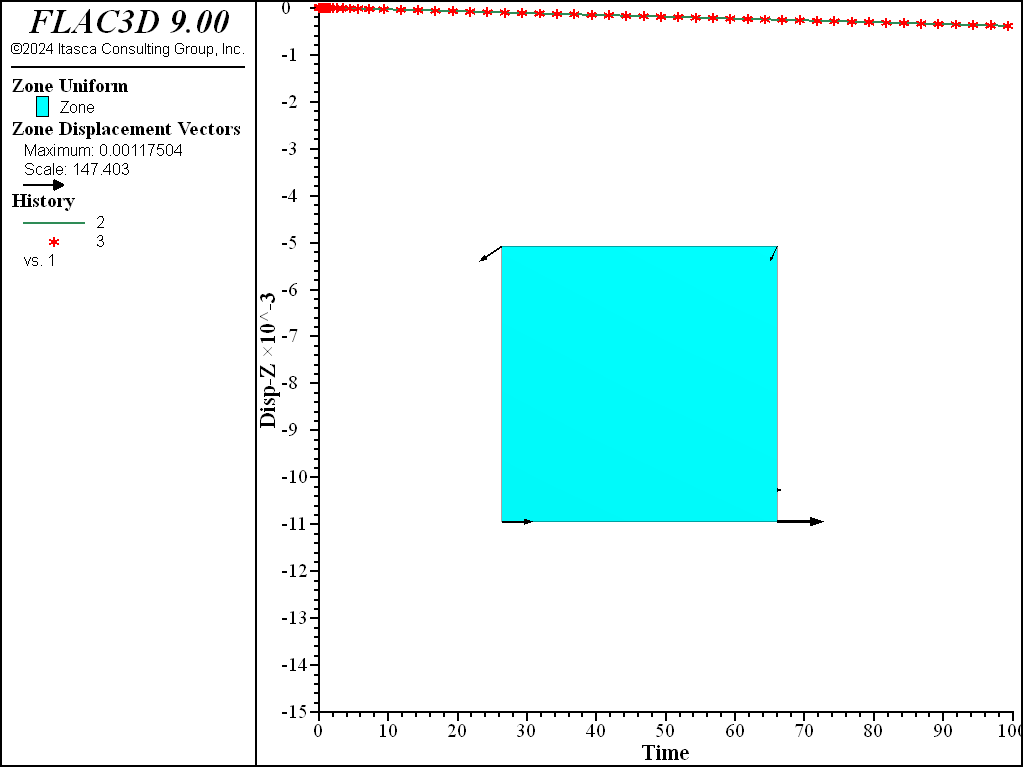
Figure 2: Final displacement vectors for dip = 15 degrees, and comparison with exact solution of vertical displacement with creep time.
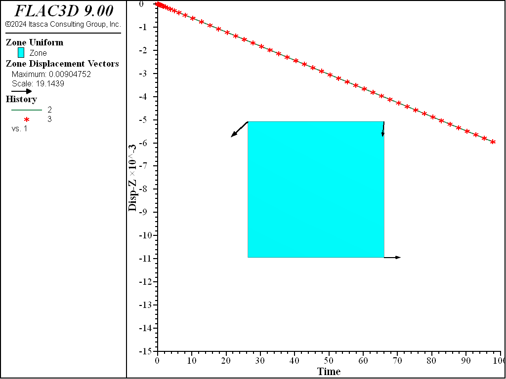
Figure 3: Final displacement vectors for dip = 30 degrees, and comparison with exact solution of vertical displacement with creep time.
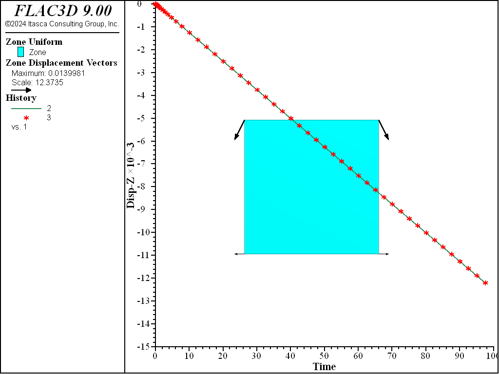
Figure 4: Final displacement vectors for dip = 45 degrees, and comparison with exact solution of vertical displacement with creep time.
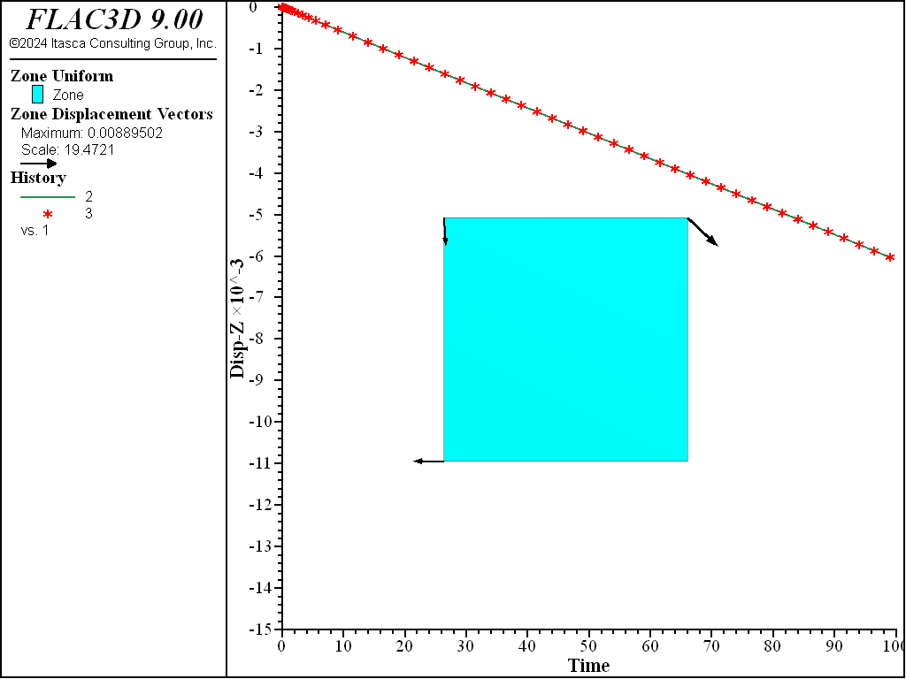
Figure 5: Final displacement vectors for dip = 60 degrees, and comparison with exact solution of vertical displacement with creep time.
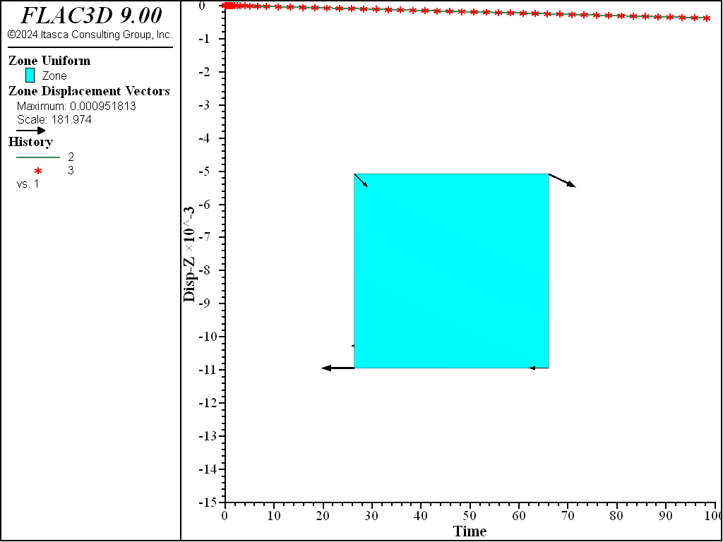
Figure 6: Final displacement vectors for dip = 75 degrees, and comparison with exact solution of vertical displacement with creep time.
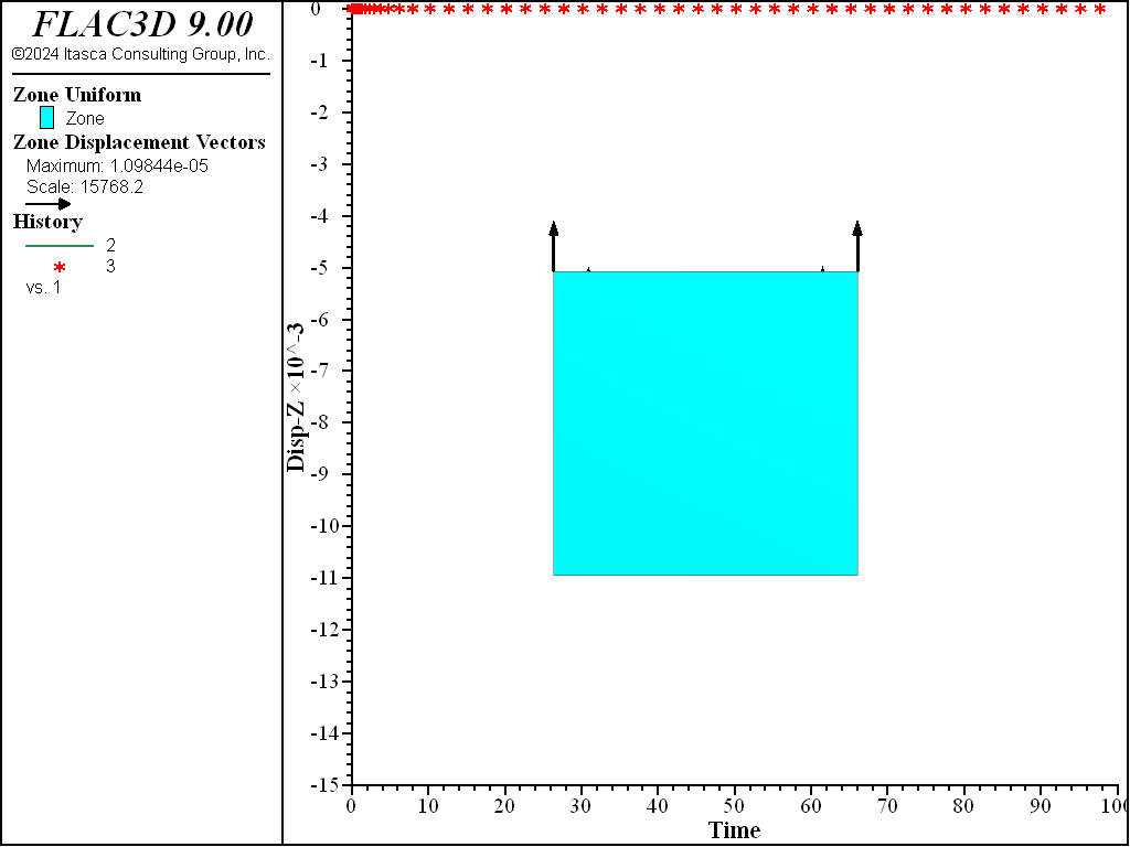
Figure 7: Final displacement vectors for dip = 0 degree, and comparison with exact solution of vertical displacement with creep time.
Data File
;----------------------------------------------------------------------
; Unconfined loading -- Comba with creep Power law in Ubiquitous joint
;----------------------------------------------------------------------
model new
fish automatic-create off
model title 'Creep element test with COMBA model'
model large-strain off
model configure creep
zone create brick size 1 1 1
;
fish define setup
    global bu    = 20.
    global sh    = 15.
    global P     = -1.
    global cons  = 1./(3.*bu) + 1./sh
    global teta1 = 15.
    ;
    global Young   = 9.*bu*sh/(3.*bu+sh)
    global Poisson = (3.*bu-2.*sh)/(6.*bu+2.*sh)
    local  alpha1  = (90. + teta1)*math.degrad
    global nx1_    = math.cos(alpha1)
    global nz1_    = math.sin(alpha1)
end
[setup]
;
zone cmodel assign columnar-basalt
zone property young [Young] poisson [Poisson]
zone property space-1 1.0 stiffness-normal-1 1.0 stiffness-shear-1 1.0
zone property normal-x-1 [nx1_] normal-y-1 0 normal-z-1 [nz1_]
zone property joint-cohesion-1 1.0 joint-friction-1 0 joint-tension-1 1e10
zone property creep-limit-ratio-1 0.0 creep-coefficient-1 0.002 creep-exponent-1 4.
zone property flag-matrix-plastic off
;
zone gridpoint fix velocity-z range position-z 0
zone face apply stress-zz [P] range position-z 1
;
program call "fish.fis"
; initial "instantaneous" equilibrium
model solve
; reset displacements and velocities
zone gridpoint initialize displacement (0,0,0)
zone gridpoint initialize velocity (0,0,0)
; --- histories ---
history interval 25
model history creep time-total
zone history displacement-z position 1 1 1
fish history dis_z
fish history tau1r
fish history taum1r
zone history stress-zz zoneid 1
fish history crerat1
; creep
model creep timestep starting 1e-8
model creep timestep automatic
model creep timestep minimum 1e-8
model creep timestep maximum 0.1
model solve creep time-total 100.
model save 'dip15'
;
| Was this helpful? ... | Itasca Software © 2024, Itasca | Updated: Nov 12, 2025 |
