Comparison of FLAC3D to SHAKE for a Layered, Linear-Elastic Soil Deposit
Note
The project file for this example is available to be viewed/run in FLAC3D. The project’s main data files are shown at the end of this example.
The program SHAKE is widely used in the field of earthquake engineering for computing the seismic response of horizontally layered soil deposits. Here, we compare FLAC3D with SHAKE (Idriss and Sun 1992) for the case of a one-dimensional layered elastic soil deposit, driven at its base by the horizontal acceleration given by the following equation,
where: |
\(\alpha\) |
= |
2.2; |
\(\beta\) |
= |
0.375; |
|
\(\gamma\) |
= |
8.0; and |
|
\(f\) |
= |
3 Hz. |
This input acceleration wave, plotted in Figure 1, shows a maximum horizontal acceleration of 0.2 g, reached after 3.75 seconds. The waveform selected for this comparison test does not require a baseline correction (see Baseline Correction); the final velocity and displacement are both zero. Neither does this form contain high-frequency components that could cause numerical distortion of the wave (see Wave Transmission).
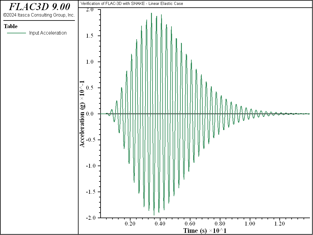
Figure 1: Input acceleration at bottom of model.
The version of SHAKE used in the comparison is SHAKE-91 (Idriss and Sun 1992). SHAKE-91 is a modified version of SHAKE, published in 1971 by the Earthquake Engineering Research Center at the University of California, Berkeley. SHAKE-91 computes the response of a semi-infinite horizontally layered soil deposit overlying a uniform half-space subjected to vertically propagating shear waves. The program performs a linear analysis in the frequency domain; an iterative procedure accounts for some of the nonlinear effects in the soil. We assume for the purposes of comparison that the soil is linear. The data file for the analysis with SHAKE-91 is shown at the end of this example.
FLAC3D is compared to SHAKE-91 for the following problem conditions. A layered soil deposit is 160 feet thick and contains two materials, as shown in Figure 2. The stiffer layer (material 2) is 40 feet thick, starts at a depth of 40 feet, and is sandwiched between the softer layers (material 1).
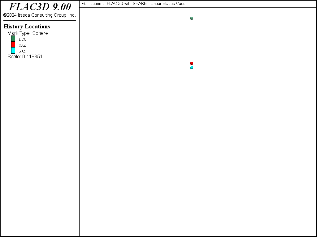
Figure 2: One-dimensional model containing two materials (history locations are also shown).
The soil is treated as a linear elastic material with the following properties:
material |
1 |
2 |
shear modulus (MPa) |
150 |
300 |
density (kg/m3) |
1800 |
2000 |
fraction of critical damping (%) |
10 |
10 |
By assuming that shear modulus and damping are strain-independent, the same properties are used in FLAC3D and SHAKE-91.
The FLAC3D model consists of 16 cubic zones, each with a height of 10 feet (3.05 m); the zone length is well within 1/10 of the longest wavelength to provide accurate wave transmission. Vertical movement is prevented at the sides of the model. Raleigh damping is specified at 10%, operating at a center frequency of 3 Hz.
Figure 3 shows the horizontal acceleration at the top of the model (gridpoint 65 in FLAC3D, and sub-layer 1 in SHAKE-91) as a function of time. Both records are very similar; the maximum acceleration calculated by FLAC3D is 0.160 g, while the maximum acceleration calculated by SHAKE-91 is 0.156 g (2.6% difference).
Figure 4 and Figure 5 show the evolution of shear strain and shear stress at a depth of 35 feet (within material 1). The FLAC3D results have been obtained through a history of \(\sigma_{xy}\) and \(\epsilon_{xy}\) at zone 13. The SHAKE-91 results have been obtained at the top of sub-layer 5 using analysis option 7 in the code. Again, the results from both codes are very similar, with a difference of less than 4%. Note that the stress histories do not contain the viscous component contributed by Rayleigh damping. This component exists in the model but cannot be plotted directly by either FLAC3D or SHAKE-91.
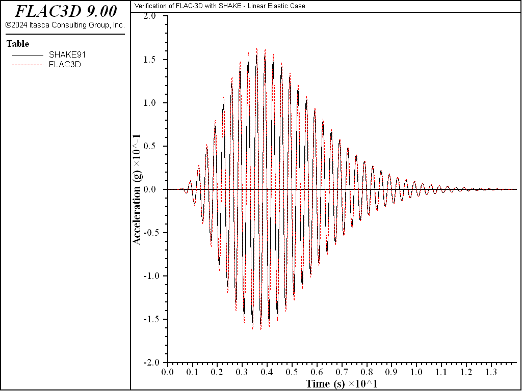
Figure 3: Horizontal acceleration at top of model.
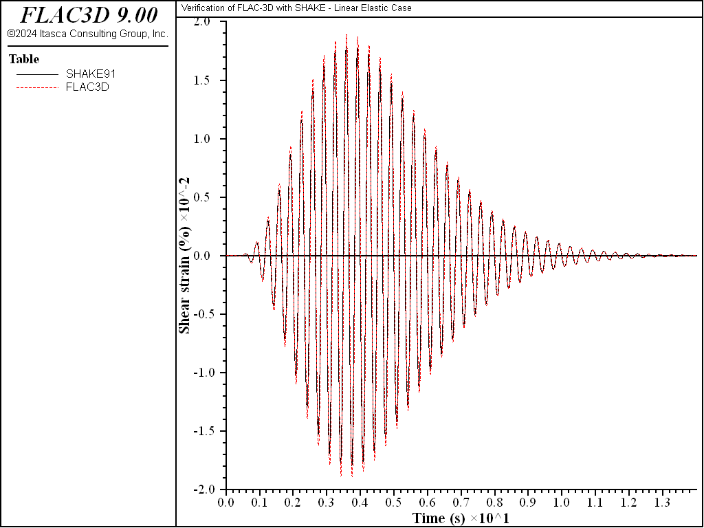
Figure 4: Shear strain history at depth of 35 ft in model.
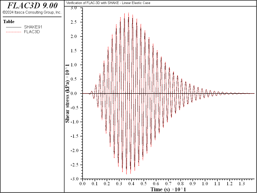
Figure 5: Shear stress history at depth of 35 ft in model.
References
Idriss, I. M., and Joseph I. Sun. User’s Manual for SHAKE-91. University of California, Davis, Center for Geotechnical Modeling, Department of Civil & Environmental Engineering (November 1992).
Data Files
F3ShakeLinearElasticCase.dat
;---------------------------------------------------------------------
;  Script file for dynamic problem 'Verification of FLAC-3D with SHAKE'
;     Linear Elastic Case, Model of Layered soil deposits
;---------------------------------------------------------------------
model new
model large-strain off
fish automatic-create off
model title "Verification of FLAC-3D with SHAKE - Linear Elastic Case"
model configure dynamic
;--- Grid generation ---
zone create brick size 1,1,16
zone gridpoint initialize position (3.048,3.048,3.048) multiply
;--- Name regions of the model ---
zone group 'material 1'
zone group 'material 2' range position-z=24.38,36.58
zone face skin
;--- Model and properties ---
zone cmodel assign elastic
zone property bulk 150e6 shear 150e6 density 1800 range group 'material 1'
zone property bulk 300e6 shear 300e6 density 2000 range group 'material 2'
;--- Boundary Conditions ---
zone gridpoint fix velocity-y range group 'Bottom' not
zone gridpoint fix velocity-z range group 'Bottom' not
fish define acc_p  ;--- FISH function to generate input wave ---
    local time = dynamic.time.total
    acc_p = math.sqrt(0.375*math.exp(-2.2*time)*time^8)* ...
                      math.sin(6.0*math.pi*time)
end
zone face apply acceleration (1,0,0) fish acc_p range group 'Bottom'
;--- Histories ---
model history name 'time' dynamic time-total
zone history name 'sxz' stress-xz position (0,0,37)
zone history name 'acc' acceleration-x position (0,0,48.768)
zone history name 'exz' strain-increment-xz position (0,0,38)
; --- Damping ---
zone dynamic damping rayleigh 0.1 3.0
;--- Solve to 14 seconds
model solve time-total 14.0
model save 'Shake'
SHAKE-91 model of layered soil deposits
option 1 - dynamic soil properties -
     1
     3
    11 material #1 modulus
0.0001 0.0003 0.001 0.003 0.01 0.03 0.1 0.3
1. 3. 10.
1.000 1.000 1.000 1.000 1.000 1.000 1.000 1.000
1.000 1.000 1.000
    11 damping for material #1
0.0001 0.0003 0.001 0.003 0.01 0.03 0.1 0.3
1. 3.16 10.
10.00 10.00 10.00 10.00 10.00 10.00 10.00 10.00
10.00 10.00 10.00
    11 material #2 modulus
0.0001 0.0003 0.001 0.003 0.01 0.03 0.1 0.3
1. 3. 10.
1.000 1.000 1.000 1.000 1.000 1.000 1.000 1.000
1.000 1.000 1.000
    11 damping for material #2
0.0001 0.0003 0.001 0.003 0.01 0.03 0.1 0.3
1. 3. 10.
10.00 10.00 10.00 10.00 10.00 10.00 10.00 10.00
10.00 10.00 10.00
     8 material #3 modulus
.0001 0.0003 0.001 0.003 0.01 0.03 0.1 1.0
1.000 1.000 1.000 1.000 1.000 1.000 1.000 1.000
     5 damping for material #3
.0001 0.001 0.01 0.1 1.
10.00 10.00 10.00 10.00 10.00
     3 1 2 3
Option 2 -- Soil Profile
     2
     1 19 Example -- 160-ft layer with 2 materials
     1 2 10.00 3130.086 .100 .11225
     2 2 10.00 3130.086 .100 .11225
     3 2 10.00 3130.086 .100 .11225
     4 2 5.00 3130.086 .100 .11225
     5 2 5.00 3130.086 .100 .11225
     6 1 5.00 6260.173 .100 .12473
     7 1 5.00 6260.173 .100 .12473
     8 1 10.00 6260.173 .100 .12473
     9 1 10.00 6260.173 .100 .12473
    10 1 10.00 6260.173 .100 .12473
    11 2 10.00 3130.086 .100 .11225
    12 2 10.00 3130.086 .100 .11225
    13 2 10.00 3130.086 .100 .11225
    14 2 10.00 3130.086 .100 .11225
    15 2 10.00 3130.086 .100 .11225
    16 2 10.00 3130.086 .100 .11225
    17 2 10.00 3130.086 .100 .11225
    18 2 10.00 3130.086 .100 .11225
    19 3 .100 .140 4000.
Option 3 -- input motion:
     3
2048 2048 .01 inp3.acc (8f10.6)
  1.0 100. 0 8
Option 4 -- sublayer for input motion (within (1) or outcropping (0)):
     4
    19 0
Option 5 -- number of iterations & ratio of avg strain to max strain
     5
    1 2 1.00
Option 6 -- sublayers for which accn time histories are computed and saved:
     6
     1 2 3 4 5 6 7 8 9 10 11 12 13 14 15
     0 1 1 1 1 1 1 1 1 1 1 1 1 1 1
     1 0 0 0 0 1 0 0 0 0 1 0 0 0 0
Option 6 -- sublayers for which accn time histories are computed and saved:
     6
    16 17 17 19 19
     1 1 1 1 0
     0 0 0 0 1
option 7 -- sublayer for which shear stress or strain are computed & saved:
     7
     5 1 1 02048 -- stress in level 5
     5 0 1 02048 -- strain in level 5
option 7 -- sublayer for which shear stress or strain are computed & saved:
     7
     7 1 1 02048 -- stress in level 7
     7 0 1 02048 -- strain in level 7
execution will stop when program encounters 0
     0
⇐ Natural Periods of an Elastic Column | Comparison of FLAC3D to SHAKE for a Layered, Nonlinear-Elastic Soil Deposit ⇒
| Was this helpful? ... | Itasca Software © 2024, Itasca | Updated: Nov 12, 2025 |
