Dynamic Modeling Considerations

There are three aspects that the user should consider when preparing a FLAC3D model for a dynamic analysis: 1) dynamic loading and boundary conditions; 2) wave transmission through the model; and 3) mechanical damping. This section provides guidance on addressing each aspect when preparing a FLAC3D data file for dynamic analysis. Solving Dynamic Problems and Verification Problems illustrate the use of most of the features discussed here.

Dynamic Loading and Boundary Conditions

FLAC3D models a region of material subjected to external and/or internal dynamic loading by applying a dynamic input boundary condition at either the model boundary or internal gridpoints. Wave reflections at model boundaries may be reduced by specifying quiet (viscous) or free-field boundary conditions. The types of dynamic loading and boundary conditions are shown schematically in Figure 1; each condition is discussed in the following sections.

Application of Dynamic Input

In FLAC3D, the dynamic input can be applied in one of the following ways:

• an acceleration history;

• a velocity history;

• a stress (or pressure) history; or

• a force history.

Dynamic input is usually applied to the model boundaries with the zone face apply command. Accelerations, velocities, and forces can also be applied to interior gridpoints by using the zone gridpoint fix command. Note that the free-field boundary, shown in Figure 1, is not required if the only dynamic source is within the model (see Free-Field Boundaries).

The history function for the input is treated as a multiplier on the value specified with the zone face apply command. The history multiplier is assigned with the history keyword and can be in one of two forms:

• a table defined by the table command; or

• a FISH function.

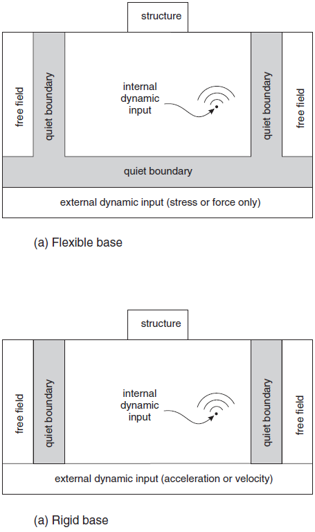
Figure 1: Types of dynamic loading and boundary conditions available in FLAC3D.

With table input, the multiplier values and corresponding time values are entered as individual pairs of numbers in the specified table; the first number of each pair is assumed to be a value of dynamic time. The time intervals between successive table entries need not be the same for all entries. The table import command allows files containing time histories (such as earthquake records) to be imported into a specified FLAC3D table. If a FISH function is used to provide the multiplier, the function must access dynamic time within the function, using the FLAC3D scalar variable zone.dynamic.time.total, and compute a multiplier value that corresponds to this time. The example of Shear Wave Propagation in a Vertical Bar provides an example of dynamic loading derived from a FISH function.

Dynamic input can be applied in the \(x\)-, \(y\)-, or \(z\)-direction corresponding to the \(x\)-, \(y\)-, \(z\)-axes for the model, or in the normal and shear directions to the model boundary.

One restriction when applying velocity or acceleration input to model boundaries is that these boundary conditions cannot be applied along the same boundary as a quiet (viscous) boundary condition (compare Figure 1-a to Figure 1-b), since the effect of the quiet boundary would be nullified. To input seismic motion at a quiet boundary, a stress boundary condition is used (i.e., a velocity record is transformed into a stress record and applied to a quiet boundary). A velocity wave may be converted to an applied stress using the formula

(1)\[\sigma_n = 2 (\rho\ C_p)\ v_n\]

or

(2)\[\sigma_s = 2 (\rho\ C_s)\ v_s\]

where:	\(\sigma_n\)	=	applied normal stress;
	\(\sigma_s\)	=	applied shear stress;
	\(\rho\)	=	mass density;
	\(C_p\)	=	speed of \(p\)-wave propagation through medium;
	\(C_s\)	=	speed of \(s\)-wave propagation through medium;
	\(v_n\)	=	input normal particle velocity; and
	\(v_s\)	=	input shear particle velocity.

\(C_p\) is given by

(3)\[C_p = \sqrt{K+4G/3\over\rho}\]

and \(C_s\) is given by

(4)\[C_s = \sqrt{G/\rho}\]

The formulae assume plane-wave conditions. The factor of two in Equations (1) and (2) accounts for the fact that the applied stress must be double that which is observed in an infinite medium, since half the input energy is absorbed by the viscous boundary. The formulation is similar to that of Joyner and Chen (1975).

The following example illustrates wave input at a quiet boundary:

• Shear Wave Propagation in a Vertical Bar

Baseline Correction

If a “raw” acceleration or velocity record from a site is used as a time history, the FLAC3D model may exhibit continuing velocity or residual displacements after the motion has finished. This arises from the fact that the integral of the complete time history may not be zero. For example, the idealized velocity waveform in Figure 2a may produce the displacement waveform in Figure 2b when integrated. The process of “baseline correction” should be performed, although the physics of the FLAC3D simulation usually will not be affected if it is not done. It is possible to determine a low frequency wave (for example, Figure 2c) which, when added to the original history, produces a final displacement that is zero (Figure 2d). The low frequency wave in Figure 2c can be a polynomial or periodic function, with free parameters that are adjusted to give the desired results. An example baseline correction function of this type is given as a FISH function in Dynamic Conditions and Simulation.

Baseline correction usually applies only to complex waveforms derived, for example, from field measurements. When using a simple, synthetic waveform, it is easy to arrange the process of generating the synthetic waveform to ensure that the final displacement is zero. Normally, in seismic analysis, the input wave is an acceleration record. A baseline-correction procedure can be used to force both the final velocity and displacement to be zero. Earthquake engineering texts should be consulted for standard baseline correction procedures.

An alternative to baseline correction of the input record is the application of a displacement shift at the end of the calculation if there is a residual displacement of the entire model. This can be done by applying a fixed velocity to the mesh to reduce the residual displacement to zero. This action will not affect the mechanics of the deformation of the model.

Computer codes to perform baseline corrections are available from several websites (for example, http://nsmp.wr.usgs.gov/processing.html).

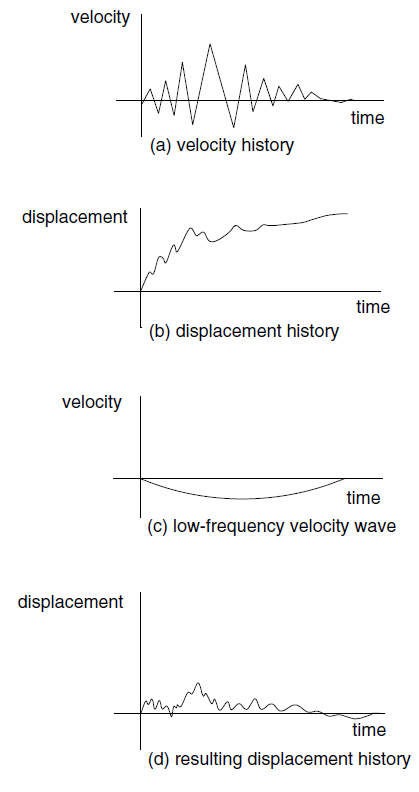
Figure 2: The baseline-correction process.

Quiet Boundaries

The modeling of geomechanics problems involves media which, at the scale of the analysis, are better represented as unbounded. Deep underground excavations are normally assumed to be surrounded by an infinite medium, while surface and near-surface structures are assumed to lie on a half-space. Numerical methods relying on the discretization of a finite region of space require that appropriate conditions be enforced at the artificial numerical boundaries. In static analyses, fixed or elastic boundaries (e.g., represented by boundary-element techniques) can be realistically placed at some distance from the region of interest. In dynamic problems, however, such boundary conditions cause the reflection of outward propagating waves back into the model, and do not allow the necessary energy radiation. The use of a larger model can minimize the problem, since material damping will absorb most of the energy in the waves reflected from distant boundaries. However, this solution leads to a large computational burden. The alternative is to use quiet (or absorbing) boundaries. Several formulations have been proposed. The viscous boundary developed by Lysmer and Kuhlemeyer (1969) is used in FLAC3D. It is based on the use of independent dashpots in the normal and shear directions at the model boundaries. The method is almost completely effective at absorbing body waves approaching the boundary at angles of incidence greater than 30°. For lower angles of incidence, or for surface waves, there is still energy absorption, but it is not perfect. However, the scheme has the advantage that it operates in the time domain. Its effectiveness has been demonstrated in both finite-element and finite-difference models (Kunar et al. 1977). A variation of the technique proposed by White et al. (1977) is also widely used.

More efficient energy absorption (particularly in the case of Rayleigh waves) requires the use of frequency-dependent elements, which can only be used in frequency-domain analyses (e.g., Lysmer and Waas 1972). These are usually termed “consistent boundaries” and involve the calculation of dynamic stiffness matrices coupling all the boundary degrees-of-freedom. Boundary-element methods may be used to derive these matrices (e.g., Wolf 1985). A comparative study of the performance of different types of elementary, viscous, and consistent boundaries was documented by Roesset and Ettouney (1977).

The quiet-boundary scheme proposed by Lysmer and Kuhlemeyer (1969) involves dashpots attached independently to the boundary in the normal and shear directions. The dashpots provide viscous normal and shear tractions given by

(5)\[t_n = - \rho\;C_p\;v_n\]

(6)\[t_s = - \rho\;C_s\;v_s\]

where \(v_n\) and \(v_s\), are the normal and shear components of the velocity at the boundary, \(\rho\) is the mass density, and \(C_p\) and \(C_s\) are the \(p\)- and \(s\)-wave velocities.

These viscous terms can be introduced directly into the equations of motion of the gridpoints lying on the boundary. A different approach, however, was implemented in FLAC3D, whereby the tractions \(t_n\) and \(t_s\) are calculated and applied at every timestep in the same way boundary loads are applied. This is more convenient than the former approach, and tests have shown that the implementation is equally effective. The only potential problem concerns numerical stability, because the viscous forces are calculated from velocities lagging by half a timestep. In practical analyses to date, no reduction of timestep has been required by the use of the nonreflecting boundaries. Timestep restrictions demanded by small zones are usually more important.

Dynamic analysis starts from some in-situ condition. If a fixed boundary is used while generating the static stress state, this boundary condition can be replaced by quiet boundaries; the boundary gridpoints will be freed, and the boundary reaction forces will beautomatically calculated and maintained throughout the dynamic loading phase. However, changes in static loading during the dynamic phase should be avoided. For example, if a tunnel is excavated after quiet boundaries have been specified on the bottom boundary, the whole model will start to move upward. This is because the total gravity force no longer balances the total reaction force at the bottom that was calculated when the boundary was changed to a quiet one.

Quiet boundary conditions can be applied in the global coordinate directions, or along inclined boundaries, in the normal and shear directions using the zone face apply command with appropriate keywords (quiet-normal, quiet-dip, quiet-strike for one component or quiet for all three components). When using the zone face apply command to install a quiet boundary condition, remember that the material properties used in Equations (5) and (6) are obtained from the zones immediately adjacent to the boundary. Thus, appropriate material properties for boundary zones must be in place at the time the zone face apply command is given, in order for the correct properties of the quiet boundary to be stored.

Quiet boundaries are best-suited when the dynamic source is within a grid. Quiet boundaries should not be used alongside boundaries of a grid when the dynamic source is applied as a boundary condition at the top or base, because the wave energy will “leak out” of the sides. In this situation, free-field boundaries (described below) should be applied to the sides.

Free-Field Boundaries

Numerical analysis of the seismic response of surface structures such as dams requires the discretization of a region of the material adjacent to the foundation. The seismic input is normally represented by plane waves propagating upward through the underlying material. The boundary conditions at the sides of the model must account for the free-field motion that would exist in the absence of the structure. In some cases, elementary lateral boundaries may be sufficient. For example, if only a shear wave were applied on the horizontal boundary, AC (shown in Figure 3), it would be possible to fix the boundary along AB and CD in the vertical direction only (see the example in Shear Wave Loading of a Model with Free-Field Boundaries). These boundaries should be placed at distances sufficient to minimize wave reflections and achieve free-field conditions. For soils with high material damping, this condition can be obtained with a relatively small distance (Seed et al. 1975). However, when the material damping is low, the required distance may lead to an impractical model. An alternative procedure is to “enforce” the free-field motion in such a way that boundaries retain their non-reflecting properties (i.e., outward waves originating from the structure are properly absorbed). This approach was used in the continuum finite-volume code NESSI (Cundall et al. 1980). A technique of this type involving the execution of free-field calculations in parallel with the main-grid analysis was developed for FLAC3D.

The lateral boundaries of the main grid are coupled to the free-field grid by viscous dashpots to simulate a quiet boundary (see Figure 3), and the unbalanced forces from the free-field grid are applied to the main-grid boundary. Both conditions are expressed in Equations (7), (8), and (9), which apply to the free-field boundary along one side-boundary plane with its normal in the direction of the \(x\)-axis. Similar expressions may be written for the other sides and corner boundaries:

(7)\[F_x=-\rho C_p(v_x^m-v_x^{\rm ff}) A + F_x^{\rm ff}\]

(8)\[F_y=-\rho C_s(v_y^m-v_y^{\rm ff}) A + F_y^{\rm ff}\]

(9)\[F_z=-\rho C_s(v_z^m-v_z^{\rm ff}) A + F_z^{\rm ff}\]

where:	\(\rho\)	=	density of material along vertical model boundary;
	\(C_p\)	=	\(p\)-wave speed at the side boundary;
	\(C_s\)	=	\(s\)-wave speed at the side boundary;
	\(A\)	=	area of influence of free-field gridpoint;
	\(v_x^m\)	=	\(x\)-velocity of gridpoint in main grid at side boundary;
	\(v_y^m\)	=	\(y\)-velocity of gridpoint in main grid at side boundary;
	\(v_z^m\)	=	\(z\)-velocity of gridpoint in main grid at side boundary;
	\(v_x^{\rm ff}\)	=	\(x\)-velocity of gridpoint in side free field;
	\(v_y^{\rm ff}\)	=	\(y\)-velocity of gridpoint in side free field;
	\(v_z^{\rm ff}\)	=	\(z\)-velocity of gridpoint in side free field;
	\(F_x^{\rm ff}\)	=	free-field gridpoint force with contributions from the \(\sigma_{xx}^{\rm ff}\) stresses of the free-field zones around the gridpoint;
	\(F_y^{\rm ff}\)	=	free-field gridpoint force with contributions from the \(\sigma_{xy}^{\rm ff}\) stresses of the free-field zones around the gridpoint; and
	\(F_z^{\rm ff}\)	=	free-field gridpoint force with contributions from the \(\sigma_{xz}^{\rm ff}\) stresses of the free-field zones around the gridpoint.

In this way, plane waves propagating upward suffer no distortion at the boundary because the free-field grid supplies conditions that are identical to those in an infinite model. If the main grid is uniform, and there is no surface structure, the lateral dashpots are not exercised because the free-field grid executes the same motion as the main grid. However, if the main-grid motion differs from that of the free field (due to, say, a surface structure that radiates secondary waves), then the dashpots act to absorb energy in a manner similar to quiet boundaries.

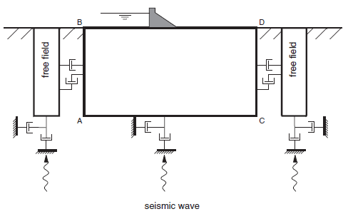
Figure 3: Model for seismic analysis of surface structures and free-field mesh.

In order to apply the free-field boundary in FLAC3D, the model must be oriented such that the base is horizontal and its normal is in the direction of the \(z\)-axis, and the sides are vertical and their normals are in the direction of either the \(x\)- or \(y\)-axis. If the direction of propagation of the incident seismic waves is not vertical, then the coordinate axes can be rotated such that the \(z\)-axis coincides with the direction of propagation. In this case, gravity will act at an angle to the \(z\)-axis, and a horizontal free surface will be inclined with respect to the model boundaries.

The free-field model consists of four plane free-field grids on the side boundaries of the model, and four column free-field grids at the corners (see Figure 4). The plane grids are generated to match the main-grid zones on the side boundaries, so that there is a one-to-one correspondence between gridpoints in the free field and the main grid. The four corner free-field columns act as free-field boundaries for the plane free-field grids. The plane free-field grids are two-dimensional calculations that assume infinite extension in the direction normal to the plane. The column free-field grids are one-dimensional calculations that assume infinite extension in both horizontal directions. Both the plane and column grids consist of standard FLAC3D zones, which have gridpoints constrained in such a way as to achieve the infinite extension assumption.

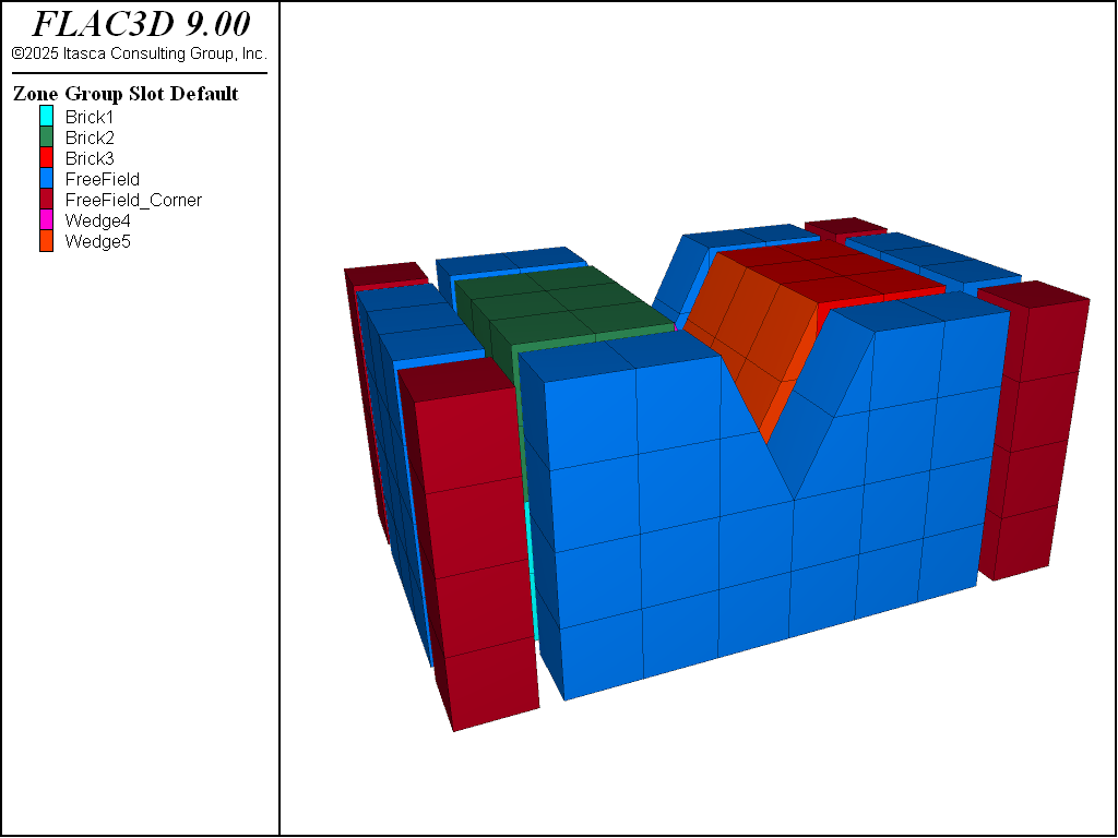
Figure 4: Side and corner free-field boundaries in a FLAC3D model.

The model should be in static equilibrium before the free-field boundary is applied. The static equilibrium conditions prior to the dynamic analysis are transferred to the free field automatically when the zone dynamic free-field command is invoked. The free-field condition is applied to lateral boundary gridpoints. All zone data (including model types and current state variables) in the model zones adjacent to the free field are copied to the free-field region. Free-field stresses are assigned the average stress of the neighboring grid zone. The dynamic boundary conditions at the base of the model should be specified before applying the free-field. These base conditions are automatically transferred to the free field when the free field is applied. Note that the free field is continuous; if the main grid contains an interface that extends to a model boundary, the interface will not continue into the free field.

After the zone dynamic free-field command is issued, the free-field grid will plot automatically whenever the main grid is plotted.

Any model or nonlinear behavior may exist in the free field, as can fluid coupling and flow within the free field.

The following is a link to a simple example of the free-field boundary in use for the model shown in Figure 4.

• Shear Wave Loading of a Model with Free-Field Boundaries

Deconvolution and Selection of Dynamic Boundary Conditions

Design earthquake ground motions developed for seismic analyses are usually provided as outcrop motions, often rock outcrop motions. [1] However, for FLAC3D analyses, seismic input must be applied at the base of the model rather than at the ground surface, as illustrated in Figure 5. The question then arises: “What input motion should be applied at the base of a FLAC3D model in order to properly simulate the design motion?”

The appropriate input motion at depth can be computed through a “deconvolution” analysis using a 1D wave propagation code such as the equivalent-linear program SHAKE or DEEPSOIL. This seemingly simple analysis is often the subject of considerable confusion resulting in improper ground motion input for FLAC3D models. The application of SHAKE for adapting design earthquake motions for FLAC3D input is described. Input of an earthquake motion into FLAC3D is typically done using one of the following:

• A rigid base, where an acceleration-time history is specified at the base of the FLAC3D mesh.

• A compliant base, where a quiet (absorbing) boundary is used at the base of the FLAC3D mesh.

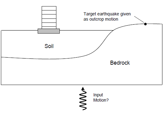
Figure 5: Seismic input to FLAC3D.

For a rigid base, a time history of acceleration (or velocity or displacement) is specified for gridpoints along the base of the mesh. While simple to use, a potential drawback of a rigid base is that the motion at the base of the model is completely prescribed. Hence, the base acts as if it were a fixed displacement boundary reflecting downward-propagating waves back into the model. Thus, a rigid base is not an appropriate boundary for general application unless a large dynamic impedance contrast is meant to be simulated at the base (e.g., low velocity sediments over high velocity bedrock).

For a compliant base simulation, a quiet boundary is specified along the base of the FLAC3D mesh. See the section on quiet boundaries. Note that if a history of acceleration is recorded at a gridpoint on the quiet base, it will not necessarily match the input history. The input stress-time history specifies the upward-propagating wave motion into the FLAC3D model, but the actual motion at the base will be the superposition of the upward motion and the downward motion reflected back from the FLAC3D model.

SHAKE (Schnabel et al. 1972) is a widely used 1D wave propagation code for site response analysis. SHAKE computes the vertical propagation of shear waves through a profile of horizontal visco-elastic layers. Within each layer, the solution to the wave equation can be expressed as the sum of an upward-propagating wave train and a downward-propagating wave train. The SHAKE solution is formulated in terms of these upward- and downward-propagating motions within each layer, as illustrated in Figure 6.

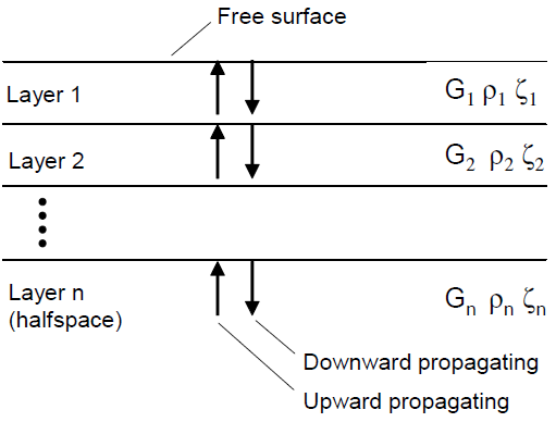
Figure 6: Layered system analyzed by SHAKE (layer properties are shear modulus, \(G\), density, \(\rho\) and damping fraction, \(\zeta\)).

The relation between waves in one layer and waves in an adjacent layer can be solved by enforcing the continuity of stresses and displacements at the interface between the layers. These well-known relations for reflected and transmitted waves at the interface between two elastic materials (Kolsky 1963) can be expressed in terms of recursion formulas. In this way, the upward- and downward-propagating motions in one layer can be computed from the upward and downward motions in a neighboring layer.

To satisfy the zero shear stress condition at the free surface, the upward- and downward-propagating motions in the top layer must be equal. Starting at the top layer, repeated use of the recursion formulas allows the determination of a transfer function between the motions in any two layers of the system. Thus, if the motion is specified at one layer in the system, the motion at any other layer can be computed.

SHAKE input and output is not in terms of the upward- and downward-propagating wave trains, but in terms of the motions at a) the boundary between two layers, referred to as a “within” motion, or b) at a free surface, referred to as an “outcrop” motion. The within motion is the superposition of the upward- and downward-propagating wave trains. The outcrop motion is the motion that would occur at a free surface at that location. Hence the outcrop motion is simply twice the upward-propagating wave-train motion. If needed, the upward-propagating motion can be computed by taking half the outcrop motion. At any point, the downward-propagating motion can then be computed by subtracting the upward-propagating motion from the within motion.

The SHAKE solution is in the frequency domain, with conversion to and from the time-domain performed with a Fourier transform. The deconvolution analysis discussed below illustrates the application of SHAKE for a linear, elastic case. See Comparison of FLAC3D to SHAKE for a Layered, Linear-Elastic Soil Deposit. SHAKE can also address nonlinear soil behavior approximately, through the equivalent linear approach. Analyses are run iteratively to obtain shear modulus and damping values for each layer that is compatible with the computed effective strain for the layer. See Comparison of FLAC3D to SHAKE for a Layered, Nonlinear-Elastic Soil.

DEEPSOIL (Hashssh et al 2017) is a one-dimensional site response analysis program that can perform: a) 1-D nonlinear time domain analyses with and without pore water pressure generation, b) 1-D equivalent linear frequency domain analyses including convolution and deconvolution, and c) 1-D linear time and frequency domain analyses.

Deconvolution for a Rigid Base — The deconvolution procedure for a rigid base is illustrated in Figure 7 for a two-dimensional FLAC simulation. The same procedure also applies to FLAC3D. The goal is to determine the appropriate base input motion to FLAC such that the target design motion is recovered at the top surface of the FLAC model. The profile modeled consists of three 20-m thick elastic layers with shear wave velocities and densities as shown in the figure. The SHAKE model includes the three elastic layers and an elastic half-space with the same properties as the bottom layer. The FLAC model consists of a column of linear elastic elements. The target earthquake is input at the top of the SHAKE column as an outcrop motion. Then, the motion at the top of the half-space is extracted as a within motion and is applied as an acceleration-time history to the base of the FLAC model. Mejia and Dawson (2006) show that the resulting acceleration at the surface of the FLAC model is virtually identical to the target motion. The SHAKE within motion is appropriate for rigid-base input because, as described above, the within motion is the actual motion at that location, the superposition of the upward- and downward-propagating waves.

Deconvolution for a Compliant Base — The deconvolution procedure for a compliant base is illustrated in Figure 8 for a FLAC simulation. Again, the same procedure applies to FLAC3D. The SHAKE and FLAC models are identical to those for the rigid body exercise, except that a quiet boundary is applied to the base of the FLAC mesh. For application through a quiet base, the upward-propagating wave motion (1/2 the outcrop motion) is extracted from SHAKE at the top of the half-space. This acceleration-time history is integrated to obtain a velocity, which is then converted to a stress history using Equation (4). Again, the resulting acceleration at the surface of the FLAC model is shown by Mejia and Dawson (2006) to be virtually identical to the target motion. As an additional check of the computed accelerations, they also show that the response spectra for both the compliant-base and rigid-base cases closely match the response spectra of the target motion.

For a deconvolution analysis, Idriss (2019 ASCE Terzaghi lecture) found that it is useful to get the strain-compatible properties by complete ting the analysis with a low cut-off frequency (say about 5 Hz, depending on the level of shaking), then using the resulting strain-compatible modulus and damping values for one iteration and desired cut-off frequency (typically 20 to 30 Hz).

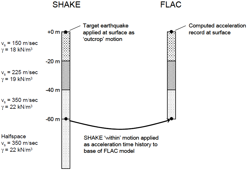
Figure 7: Deconvolution procedure for a rigid base (after Mejia and Dawson 2006).

Figure 8: Deconvolution procedure for a compliant base (after Mejia and Dawson 2006).

Although useful for illustrating the basic ideas behind deconvolution, the previous example is not the typical case encountered in practice. The situation shown in Figure 9, where one or more soil layers (expected to behave nonlinearly) overlay bedrock (assumed to behave linearly), is more common. A FLAC or FLAC3D model for this case will usually include the soil layers and an elastic base of bedrock. To compute the correct FLAC3D compliant base input, a SHAKE model is constructed as shown in the figure. The SHAKE model includes a bedrock layer equal in thickness to the elastic base of the FLAC3D mesh, and an underlying elastic half-space with bedrock properties. The target motion is input to the SHAKE model as an outcrop motion at the top of the bedrock (point A). Designating this motion as outcrop means that the upward-propagating wave motion in the layer directly below point A will be set equal to 1/2 the target motion. The upward-propagating motion for input to FLAC3D is extracted at point B as 1/2 the outcrop motion.

For the compliant-base case, there is actually no need to include the soil layers in the SHAKE model, as these will have no effect on the upward-propagating wave train between points A and B. In fact, for this simple case, it is not really necessary to perform a formal deconvolution analysis, as the upward-propagating motion at point B will be almost identical to that at point A. Apart from an offset in time, the only differences will be due to material damping between the two points, which will generally be small for bedrock. Thus, for this very common situation, the correct input motion for FLAC3D is simply 1/2 of the target motion. (Note that the upward-propagating wave motion must be converted to a stress-time history using Equation (4), which includes a factor of 2 to account for the stress absorbed by the viscous dashpots.)

For a rigid-base analysis, the within motion at point B is required. Since this within motion incorporates downward-propagating waves reflected off the ground surface, the nonlinear soil layers must be included in the SHAKE model. However, soil nonlinearity will be modeled quite differently in FLAC3D and SHAKE. Thus, it is difficult to compute the appropriate FLAC3D input motion for a rigid-base analysis.

Another typical case encountered in practice is illustrated in Figure 10. Here, the soil profile is deep, and rather than extending the FLAC3D mesh all the way down to bedrock, the base of the model ends within the soil profile. Note that the mesh must be extended to a depth below which the soil response is essentially linear. Again, the design motion is input at the top of the bedrock (point A) as an outcrop motion, and the upward-propagating motion for input to FLAC3D is extracted at point B. As in the previous example, for a compliant-base analysis there is no need to include the soil layers above point B in the SHAKE model. These layers have no effect on the upward-propagating motion between points A and B. Unlike the previous case, the upward-propagating motion can be quite different at points A and B, depending on the impedance contrast between the bedrock and linear soil layer. Thus, it is not appropriate to skip the deconvolution analysis and use the target motion directly.

A rigid base is only appropriate for cases with a large impedance contrast at the base of the model. However, the use of SHAKE to compute the required input motion for a rigid base of a FLAC3D model leads to a good match between the target surface motion and the surface motion computed by FLAC3D only for a model that exhibits a low level of nonlinearity. The input motion already contains the effect of all layers above the base, because it contains the downward-propagating wave.

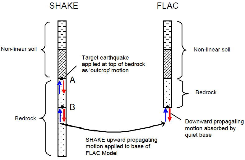
Figure 9: Compliant-base deconvolution procedure for a typical case (after Mejia and Dawson 2006).

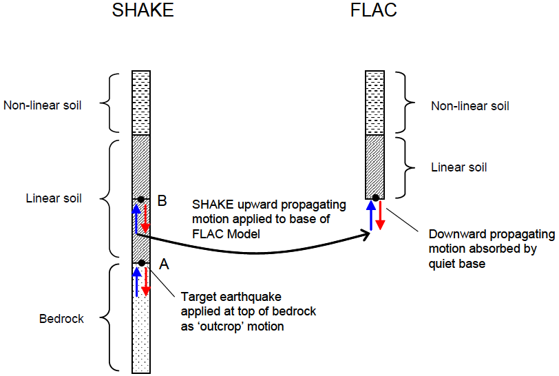
Figure 10: Compliant-base deconvolution procedure for another typical case (after Mejia and Dawson 2006).

A different approach must be taken if a FLAC3D model with a rigid base is used to simulate more realistic systems (e.g., sites that exhibit strong nonlinearity, or the effect of a surface or embedded structure). In the first case, the real nonlinear response is not accounted for by SHAKE in its estimate of base motion. In the second case, secondary waves from the structure will be reflected from the rigid base, causing artificial resonance effects.

A compliant base is almost always the preferred option because downward-propagating waves are absorbed. In this case, the quiet-base condition is selected, and only the upward-propagating wave from SHAKE is used to compute the input stress history. By using the upward-propagating wave only at a quiet FLAC3D base, no assumptions need to be made about secondary waves generated by internal nonlinearities or structures within the grid, because the incoming wave is unaffected by these; the outgoing wave is absorbed by the compliant base.

Although the presence of reflections from a rigid base is not always obvious in complex nonlinear FLAC3D analyses, they can have a major impact on analysis results, especially when cyclic-degradation or liquefaction-soil models are employed. Mejia and Dawson (2006) present examples from two-dimensional FLAC simulations that illustrate the nonphysical wave reflections calculated in models with a rigid base. One example, shown in Figure 11, demonstrates the difficulty with a rigid boundary. The nonphysical oscillations that result from a rigid base are shown by comparison to results for a compliant base in Figure 12. The inputs in both cases (rigid and compliant) were derived by deconvoluting the same surface motion.

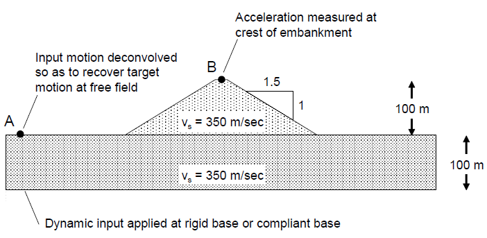
Figure 11: Embankment analyzed with a rigid and compliant base (after Mejia and Dawson 2006).

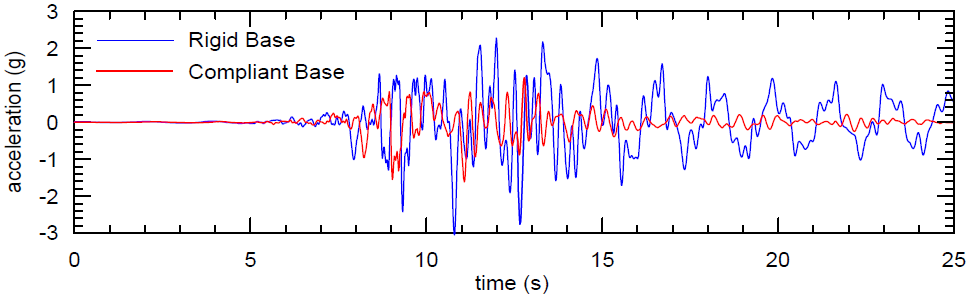
Figure 12: Computed accelerations at crest of embankment (after Mejia and Dawson 2006).

Hydrodynamic Pressures

The dynamic interaction between water in a reservoir and a concrete dam can have a significant influence on the performance of the dam during an earthquake. Westergaard (1933) established a mathematical basis for procedures to represent this interaction, and this approach is commonly used in engineering practice. Although the advent of computers has enabled numerical solution of coupled differential equations of fluid-structure systems, the formula proposed by Westergaard is widely used for stability analysis of smaller dams and preliminary calculations in the design of large dams.

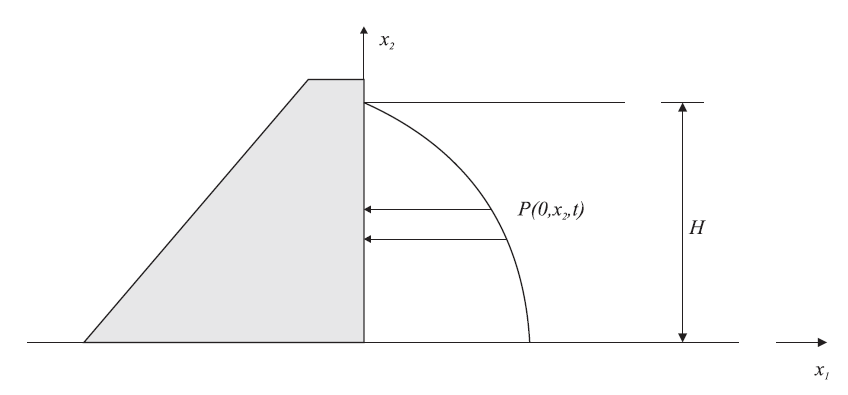
Figure 13: Hydrodynamic pressure acting on a rigid dam with a vertical upstream face.

The hydrodynamic pressure acting on a rigid concrete dam over a reservoir height, \(H\), is depicted in Figure 13. The pressure can be derived from the equation of motion for a fluid. The equation of motion for a fluid with small Reynold’s number can be written as

(10)\[c^2 \left( \frac{\delta^2 \Phi}{\delta x_1^2} + \frac{\delta^2 \Phi}{\delta x_2^2} \right) = \frac{\delta^2 \Phi}{\delta t^2}\]

where \(c\) is the speed of sound in water and \(\Phi\) is the velocity potential. The water pressure can be written as a function of the velocity potential:

\[p = \rho_w \frac{\delta \Phi}{\delta t}\]

where \(\rho_w\) is the density of water.

Additional assumptions are made to simplify the loading condition:

• The water is assumed to be incompressible, which reduces Equation (10) to the Laplace equation: \(\frac{\delta^2 \Phi}{\delta x_1^2} + \frac{\delta^2 \Phi}{\delta x_2^2} = 0\).

• The free surface of the reservoir is assumed to be at rest. Thus, \(\frac{\delta \Phi}{\delta t} = 0\) at \(x_2 = H\).

• The reservoir is assumed to be infinitely long. Therefore, as \(x_1 \rightarrow \infty, \Phi \rightarrow 0\).

• Hydrodynamic motion is assumed to be horizontal only: \(\frac{\delta \Phi}{x_2} = 0\) at \(x_2 = 0\).

• The upstream face of the dam is vertical and the dam is rigid: \(\frac{\delta \Phi}{x_1} = f(t)\) at \(x_1 = 0\).

The solution of Equation (10) with the preceding assumptions can be obtained for an arbitrary acceleration, \(\ddot{x}_0 (t)\), in the form of an infinite Fourier series:

(11)\[p(0,x_2,t) = 8 \ddot{x}_0 \rho_w H \sum_{n=1}^{\infty} \frac{(-1)^{n+1}}{((2n-1)\pi)^2}\;e^{\frac{-(2n-1)x_1}{4H}} \cos\big(\frac{(2n-1)x_2}{4H})\]

Equation (11) can be approximated as

(12)\[p(0,x_2,t) = \rho_w \ddot{x}_0(t) H \frac{C_m}{2} \left( 1 - \frac{x^2_2}{H^2} + \sqrt{1-\frac{x^2_2}{H^2}} \right)\]

where \(C_m\) = 0.743 and \(\ddot{x}\) is the horizontal acceleration at the dam face.

Equation (12) is implemented in FLAC3D by adjusting the grid point mass on the upstream face of the dam to account for the hydrodynamic pressure. The equivalent pressure, \(\bar{p}\), resulting from the inertial forces associated with the gridpoint and the hydrodynamic pressure of the water in the reservoir, averaged over the area associated with the gridpoint, can be written as

\[\bar{p}(0,x_2,t) = \rho_e\;c\;\ddot{x}_0 (t) \frac{A_g}{\Delta x_2}\]

where \(A_g\) is the area associated with the gridpoint, \(\Delta x_2\) is the contact length on the upstream face of the dam through which the water load is applied for the gridpoint, and \(\rho_ec\) is the equivalent density of the gridpoint and is given by

\[\rho_ec = \rho_c + \rho_sc\]

where

(13)\[\rho_sc = \rho_w \frac{H \delta x_2}{A_g} \frac{C_m}{2} \left( 1 - \frac{x^2_2}{H_2} + \sqrt{1 - \frac{x^2_2}{H^2}} \right)\]

\(\rho_c\) is the density of concrete such that the gridpoint mass is given by \(m_g = A_g \rho_c\). The scaled gridpoint mass, \(m_sg = A_g \rho_ec\), is used only for the motion calculation in the horizontal direction; the effect of the increase mass does not influence the vertical forces.

The gridpoint mass is adjusted by adding the term (as determined by Equation (13)) to account for the hydrodynamic pressure. This adjustment is stored in a location that is modifiable using the FISH gridpoint function gp.mass.add. The conditions are applied using the zone face westergaard command.

The following simple example is provided that illustrates the effect of hydrodynamic pressures and compares the Westergaard approximation to the result of explicitly modeling the water using FLAC3D zones.

• Hydrodynamic Pressure Acting on a Dam

Wave Transmission

Accurate Wave Propagation

Numerical distortion of the propagating wave can occur in a dynamic analysis as a function of the modeling conditions. Both the frequency content of the input wave and the wave speed characteristics of the system will affect the numerical accuracy of wave transmission. Kuhlemeyer and Lysmer (1973) show that, for accurate representation of wave transmission through a model, the spatial element size, \(\Delta l\), must be smaller than approximately one-tenth to one-eighth of the wavelength associated with the highest frequency component of the input wave. For instance,

(14)\[\Delta l \le {\lambda \over 10}\]

where \(\lambda\) is the wavelength associated with the highest frequency component that contains appreciable energy.

Filtering

For dynamic input with a high peak velocity and short rise time, the Kuhlemeyer and Lysmer requirement may necessitate a very fine spatial mesh and a corresponding small timestep. The consequence is that reasonable analyses may be prohibitively time- and memory-consuming. In such cases, it may be possible to adjust the input by recognizing that most of the power for the input history is contained in lower-frequency components (e.g., use “fft.fis” in “datafiles\FISH\Library”). By filtering the history and removing high frequency components, a coarser mesh may be used without significantly affecting the results.

The filtering procedure can be accomplished with a low-pass filter routine such as the fast Fourier transform technique. For example, the unfiltered velocity record shown in Figure 14 represents a typical waveform containing a very high frequency spike. The highest frequency of this input exceeds 50 Hz but, as shown by the power spectral density plot of Fourier amplitude versus frequency (Figure 15), most of the power (approximately 99%) is made up of components of frequency 15 Hz or lower. It can be inferred, therefore, that by filtering this velocity history with a 15 Hz low-pass filter, less than 1% of the power is lost. The input filtered at 15 Hz is shown in Figure 16, and the Fourier amplitudes are plotted in Figure 17. The difference in power between unfiltered and filtered input is less than 1%, while the peak velocity is reduced 38%, and the rise time is shifted from 0.035 to 0.09 seconds. Analyses should be performed with input at different levels of filtering to evaluate the influence of the filter on model results.

If a simulation is run with an input history that violates Equation (14), the output will contain spurious “ringing” (superimposed oscillations) that are nonphysical. The input spectrum must be filtered before being applied to a FLAC3D grid. This limitation applies to all numerical models in which a continuum is discretized; it is not just a characteristic of FLAC3D. Any discretized medium has an upper limit to the frequencies that it can transmit, and this limit must be respected for the results to be meaningful. Users of time-domain codes commonly apply sharp pulses or step waveforms to the numerical grid; this is not acceptable, since these waveforms have spectra that extend to infinity. It is a simple matter to apply, instead, a smooth pulse that has a limited spectrum. Alternatively, artificial viscosity may be used to spread sharp wave-fronts over several zones (see Artificial Viscosity), but this method strictly only applies to isotropic strain components.

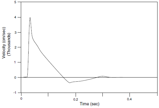
Figure 14: Unfiltered velocity history.

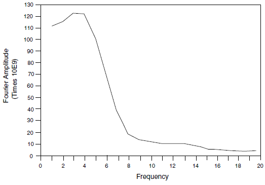
Figure 15: Unfiltered power spectral density plot.

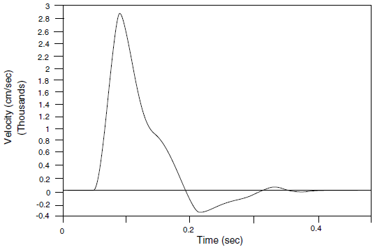
Figure 16: Filtered velocity history at 15 Hz.

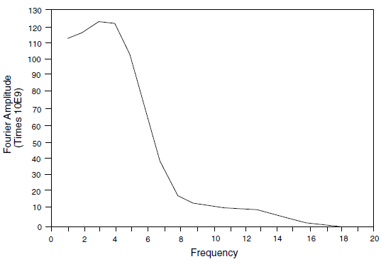
Figure 17: Results of filtering at 15 Hz.

Endnotes

[1]

This section is abstracted with permission from the publication by Mejia and Dawson (2006).

[2]

A spectral analysis based on a fast Fourier transform is supplied as a FISH function in the FISH library – see “FFT.FIS.”