Pillar Loads at Intersecting Tunnels (FLAC3D)

Problem Statement

Note

The project file for this example is available to be viewed/run in FLAC3D.[1] The project’s main data file is shown at the end of this example.

The mine layout shown in Figure 1 is representative of the production level in a mass-caving mining operation. The roadways are usually developed ahead of the mining and are initially subjected to the in-situ stress state. As mining progresses, the pillars are submitted to an increased vertical load.

The purpose of this example is to first study the initial response of the excavation (under in-situ stresses), and to then establish the peak load the pillars can carry. Also to be determined is how much stronger this pillar is than a square pillar of the same width and height.

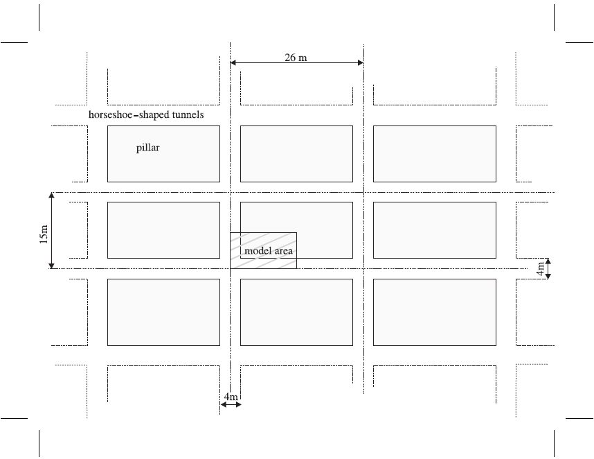
Figure 1: Mine layout.

break

The initial stress state considered is

\(σ_{xx}\) = 25 MPa (east-west)

\(σ_{yy}\) = 30 MPa (north-south)

\(σ_{zz}\) = 17 MPa (vertical)

The rock mass material properties are found in Table 1.

Table 1: Rock Mass Material Properties

bulk modulus	14.1 GPa
shear modulus	8.9 GPa
friction angle	35° (peak)
cohesion	4 MPa (peak)
dilation angle	5°
tensile strength	0.5 MPa

The rock mass is fair to good quality mass (Geologic Strength Index, \(GSI \approx\) 70) and behaves as a strain-softening material with a 0.5% critical plastic shear strain and a total loss of cohesion and a drop in friction angle of five degrees after a 2% plastic shear strain assuming the resolution of the pillar (number of zones along the pillar height) is 20.

Modeling Procedure

The FLAC3D model was used to study a quarter-section of a pillar as a result of symmetry considerations, as indicated in Figure 1. Figure 2 shows the final grid created using the built-in building-blocks block create tool of FLAC3D.

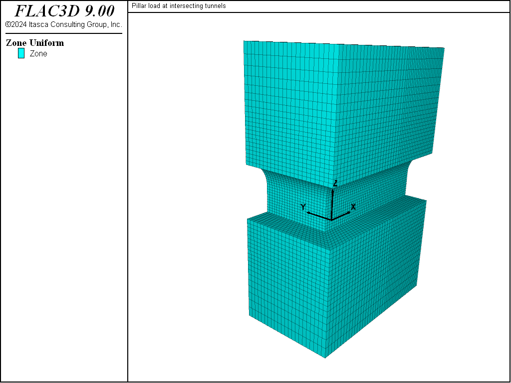
Figure 2: Final model grid.

The boundary conditions for the initial response are roller boundaries along the sides and bottom of the model, and an applied vertical stress of 17 MPa at the top of the model. In order to establish the peak load the pillar can carry, the vertical velocity of the top of the model is fixed at a constant value of -4 × 10^-6 m/step. The sum of the reaction forces at the base of the model is obtained via the FISH function s_base.

The data file for this problem, “pillar.dat”, is listed at the end of this section.

Results

Figure 3 shows contours of Z displacements after the excavation of the tunnels. As expected, most of the floor heave (about 5.1 mm) and crown displacement (about 8.2 mm) takes place at the intersection. Figure 4 shows the state of plasticity at mid-height of the pillar. The extent of the failed zones ranges from 67 cm in the center of the pillar to 1.5 m in the intersection. Figure 5 shows contours of vertical stresses at mid-height of the pillar. The vertical stresses in this plane are close to the minimum principal stresses, i.e., greatest negative stress, \(σ_1\)), so the greatest compressive stresses are located in proximity to the boundary of the plastic region near the corner of the pillar. Figure 6 shows contours of the minimum principal stress inside the pillar. At this point, the core of the pillar is relatively unstressed, and the stress concentrations around the tunnels are the most prominent feature.

At this point, the pressure boundary condition at the top of the model is replaced with a velocity boundary condition. Figure 7 shows the evolution of the average vertical stress on the base (i.e., the sum of the vertical reaction forces at the base of the model divided by the area of the base: 13 m × 7.5 m). Note that the average vertical stress in the pillar will be larger by a factor, \(F\), equal to

\[F = {13 \times 7.5 \over 11 \times 5.5} = 1.61\]

The peak average vertical stress on the base is approximately 31.9 MPa, so the peak average vertical stress in the pillar is 51.4 MPa.

The stresses in the pillar are compared when submitted to an average vertical stress on the base of 29 MPa before and after the peak stress. Figure 8 and Figure 9 show the extent of failure before and after peak. Note that roughly 30% of the cross-section of the pillar remains elastic after the peak stress has been reached. This is consistent with observations made by Wagner (1980). Figure 10 and Figure 11 show contours of vertical stress before and after peak. Even though the average vertical stress in the pillar is the same for both figures, the greatest compressive stress is higher and the de-stressed area is larger after peak.

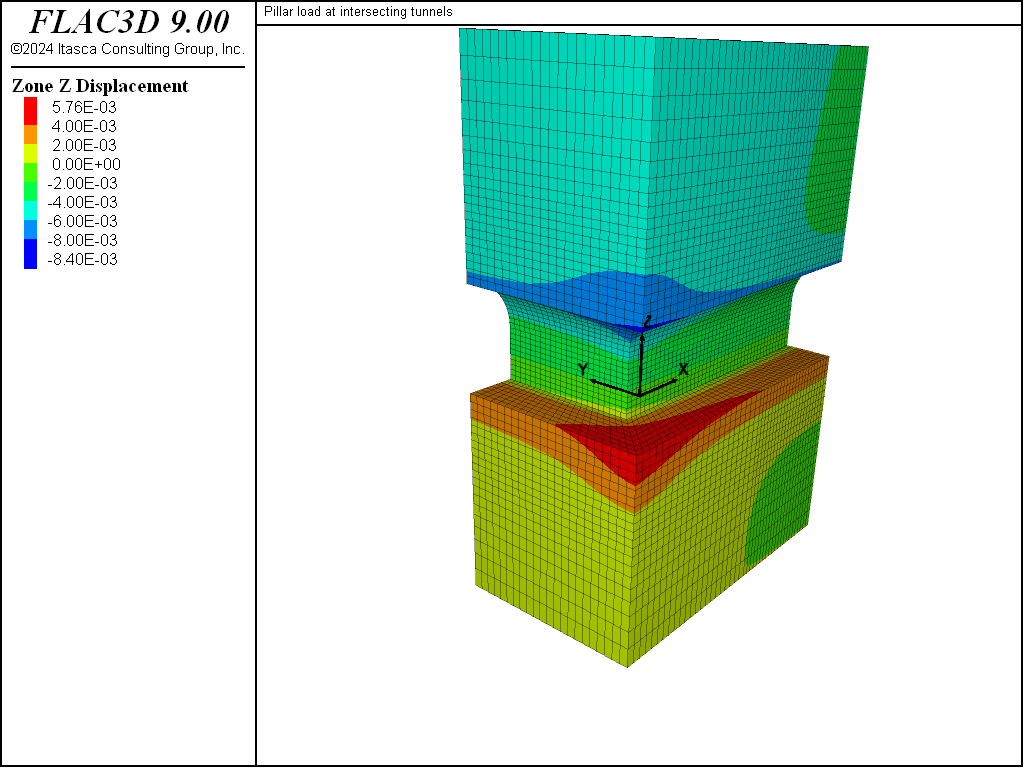
Figure 3: Displacement contours after excavation of tunnels.

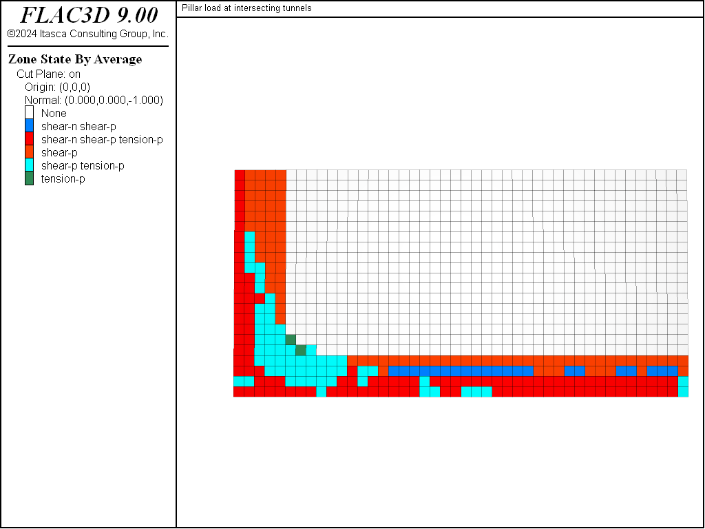
Figure 4: Plasticity state at pillar mid-height after excavation of tunnels.

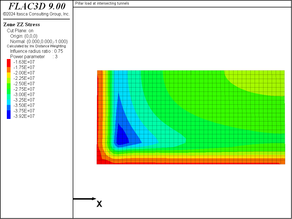
Figure 5: Vertical stress contours at pillar mid-height after excavation of tunnels.

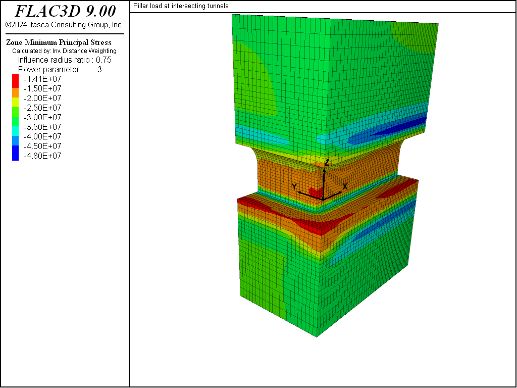
Figure 6: Minimum principal stress contours in pillar after excavation of tunnels.

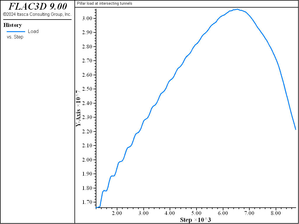
Figure 7: History of the average vertical stress on the base.

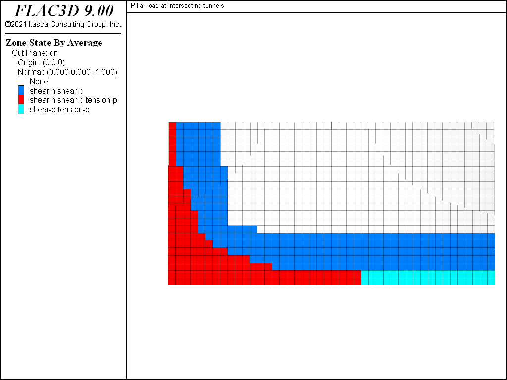
Figure 8: Plasticity state in pillar at 29 MPa average vertical stress, before peak stress.

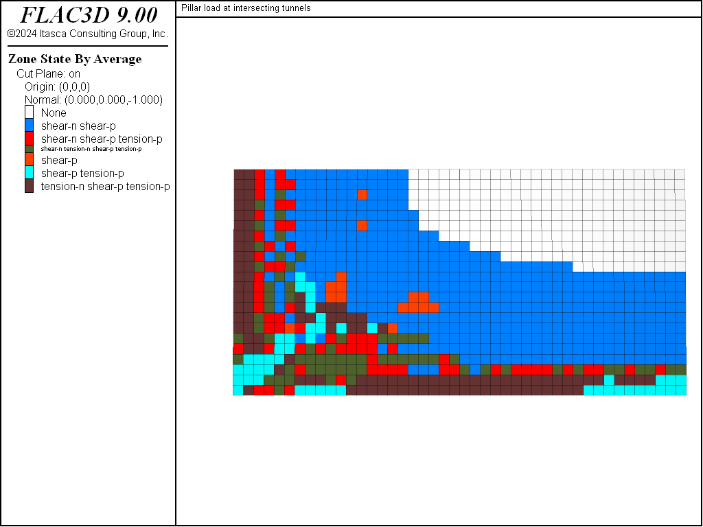
Figure 9: Plasticity state in pillar at 29 MPa average vertical stress, after peak stress.

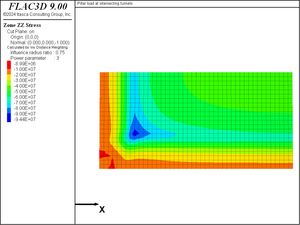
Figure 10: Vertical stress contours at 29 MPa average vertical stress, before peak stress.

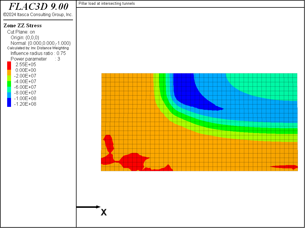
Figure 11: Vertical stress contours at 29 MPa average vertical stress, after peak stress.

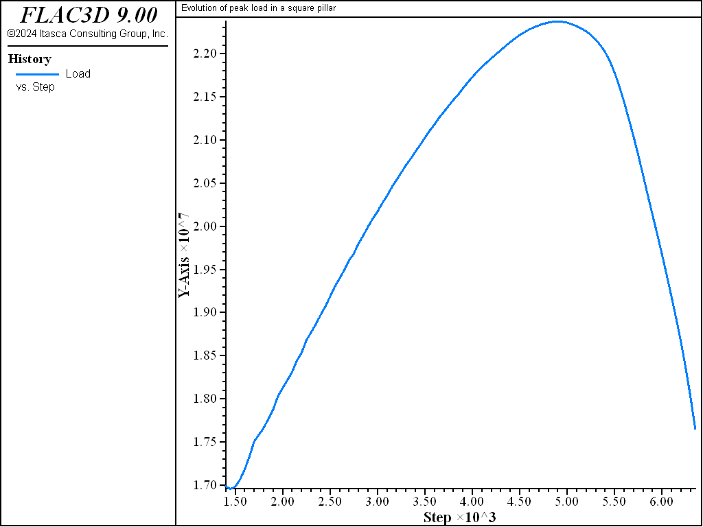
Figure 12: History of the average vertical stress on the base for a square pillar.

Discussion

Pillar Strength

Many of the published pillar strength formulae are usually expressed by an empirical power relation of the form

\[S = k V^{a} R^{b}\]

in which \(k\) is a strength parameter, \(V\) is the pillar volume, \(R\) is the width/height ratio of the pillar, and \(a\) and \(b\) are empirical parameters.

These expressions are based on square pillars and do not take into account the length of the pillar. Wagner (1980) defined an effective width for irregular pillars as

\[w_{e} = {4 A \over C}\]

in which \(A\) is the operating area and \(C\) is the pillar’s perimeter. For rectangular pillars, the effective width is

\[w_{e} = {2 w l \over w + l}\]

in which \(w\) is the width and \(l\) is the length of the pillar. Using these equations, it can be established that a rectangular pillar will be stronger than a square pillar of the same width and height by a factor, \(F_p\), of

\[F_{p} = \left({l \over w}\right)^a \cdot \left({2 \cdot l \over w + l}\right)^b\]

This equation, along with the values of \(a\) and \(b\) published by different authors, can be used to predict the strength of a square pillar.

Table 2: Predicted Square-Pillar Strength

Source	a (m)	b (m)	Predicted Strength (MPa)
Salamon and Munro (1967)	-0.067	0.59	44.11
Greenwood et al. (1939)	-0.111	0.72	43.81
Holland and Gaddy (1957)	-0.167	0.83	44.12

The data file pillar-sq.dat models one-eighth of a square pillar with the same properties and initial stress conditions as the rectangular pillar studied earlier. Figure 12 shows the evolution of the vertical stress at the base of this model. The peak stress in the pillar will be

\[\sigma_{p} = 23.6 \cdot {15 \cdot 15 \over 11 \cdot 11} = 43.9 \hbox{ MPa }\]

which compares favorably with the strength predicted using Wagner’s approach.

Grid Dependency

A strain-softening material is more prone to produce shear bands (localization). The shear bands in FLAC3D collapse down to the smallest width that can be resolved by the grid, which is one grid-width if the band is parallel to the grid, or about three grid-widths if the band cuts across the grid at an arbitrary angle. Although the overall physics of band formation is modeled correctly by FLAC3D, band thickness and band spacing are grid-dependent. Furthermore, if the strain-softening model is used with a weakening material, the load/displacement relation generated by FLAC3D for a simulated test is strongly grid-dependent. This is because the strain concentrated in a band depends on the width of the band (in length units), which depends on zone size, as previously seen. Hence, smaller zones lead to more softening, because we move out more rapidly on the strain axis of the given softening curve. To correct this grid-dependence, some sort of length scale must be built into the constitutive model. There is controversy, at present, concerning the best way to do this. It must be recognized that the grid size and angle affect the results: models must be calibrated for each grid used.

In the absence of data for calibration, a critical plastic shear strain of \(\gamma^{crit}_{p}\) = 0.5% is suggested as a starting point for modeling high-quality, massive, in-situ rock with few widely spaced discontinuities and fair to good joint conditions (\(GSI \approx\) 70). This value of strain assumes that approximately 20 zones are used to resolve the critical dimension controlling stability within the numerical model (e.g., pillar height). If a different resolution (\(R\)) than 20 zones is used, this critical strain value should be scaled by a factor of \(R\)/20. A minimum resolution of 10~15 zones is recommended for detailed studies of rock mass performance. If a lower or higher quality rock mass is to be modeled, this critical strain value should be scaled by a factor of \((10-0.1 \times GSI)/3\). Caution should be used when simulating rock masses of very high quality (\(GSI\) > 90) due to instabilities that can arise from the use of perfect (or near-perfect) brittleness. In summary, the recommended starting point for critical plastic shear strain is:

\[\gamma^{crit}_{p} = 0.5\% \times {R \over 20} \times {{10 - 0.1 \times GSI} \over 3}\]

In this example, both models are assuming fair to good quality mass (\(GSI \approx\) 70). The model by the data file “pillar-sq.dat” is with uniform zones (\(R\) = 20) so the softening rate does not need to be scaled. However, the model by the data file “pillar.dat” is with irregular zones. It is hard to use the scaling equation in a straightforward manner, but its equivalent resolution is between 16 and 20, so the softening rate is scaled by a factor of 0.9 by assuming \(R\) = 18.

More detailed discussions on grid dependency of a softening model for a generalized case are in <link to location in the User’s Guide section>. the link in the preceding needs to be built; section being linked to needs to be written/updated.

References

Greenwald, H. P., H. C. Howarth and I. Hartmann. “Experiments on Strength of Small Pillars of Coal of the Pittsburgh Bed,” U.S. Bureau of Mines, Technical Paper No. 605 (1939).

Holland, C. J., and F. L. Gaddy. “Some Aspects of Permanent Support of Overburden on Coal Beds,” in Proceedings of the West Virginia Coal Mining Institute, pp. 43-66 (1957).

Salamon, M. D. G., and A. H. Munro. “A Study of the Strength of Coal Pillars,” J. S. Afr. Inst. Min. Metall., 68, 55-67 (1967).

Wagner, H. “Pillar Design in Coal Mines,” J. S. Afr. Inst. Min. Metall., 81, 37-45 (1980).

break

Data Files

pillar.dat

;-------------------------------------------------------------
; evolution of peak load in a rectangular pillar
;-------------------------------------------------------------
model new
model configure cluster
model large-strain off
fish automatic-create off
model title 'Pillar load at intersecting tunnels'
; Model geometry - created with building-blocks and exported from state pane
program call 'geometry' 
zone generate from-building-blocks
zone face skin
; Constitutive model and properties
zone cmodel assign strain-softening
zone property bulk 14.1e9 shear 8.87e9 tension 5e5 friction 35 ...
              cohesion 4e6 dilation 5 table-friction 'fric' ...
              table-cohesion 'coh'
table 'fric' add (0, 35) (0.0045, 35) (0.018,30) (1,30)
table 'coh'  add (0,4e6) (0.0045,4e6) (0.018, 0) (1, 0)
; Initialize stresses
zone initialize stress xx -25e6 yy -30e6 zz -17e6
; Boundary conditions
zone face apply velocity-normal 0 range group 'West1' or 'West2' ...
                                           or 'East' or 'South1' ...
                                           or 'South2' or 'North' ...
                                           or 'Bottom1'
zone face apply stress-normal -17e6 range group 'Top2'
; Solve for initial excavation
model solve ratio-local 1e-3
model save 'pillar1'
; Apply velocity to top, take history of pillar load
zone face apply velocity-normal -4e-6 range group 'Top2'
[global dim1 = 13.0]
[global dim2 =  7.5]
program call 'pillar-load'
history interval 50
fish history name 'load' [load]
model step 4000 ; -1.6e-2 total top displacement
model save 'pillar2'
model step 3600 ; -3.04e-2 total top displacement
model save 'pillar3'

pillar-sq.dat

;-------------------------------------------------------------
; evolution of peak load in a square pillar
;-------------------------------------------------------------
model new
model configure cluster
model large-strain off
fish automatic-create off
model title 'Evolution of peak load in a square pillar'
; Create geometry, in this case simple to use zone create
zone create brick size (22,22,10) point 0 (2,2, -2) point 1 (7.5,2, -2) ...
                                  point 2 (2,7.5, -2) point 3 (2,2,0)
zone create brick size (30,30,10) point 0 (0,0, -5) point 1 (7.5,0, -5) ...
                                  point 2 (0,7.5, -5) point 3 (0,0,-2)
zone create brick size (30,30,10) point 0 (0,0,-10) point 1 (7.5,0,-10) ...
                                  point 2 (0,7.5,-10) point 3 (0,0,-5) ...
                                  ratio 1 1 0.9
zone face skin ; Name model boundaries
; Assign constitutive model and properties
zone cmodel assign strain-softening
zone property bulk 14.1e9 shear 8.87e9 tension 5e5 friction 35 ...
              cohesion 4e6 dilation 5 table-friction 'fric' ...
              table-cohesion 'coh'
table 'fric' add (0, 35) (0.0045, 35) (0.018,30) (1,30)
table 'coh'  add (0,4e6) (0.0045,4e6) (0.018, 0) (1, 0)
; Initialize stresses
zone initialize stress xx -25e6 yy -30e6 zz -17e6
; Boundary conditions
zone face apply velocity-normal 0 range group 'West2' or 'East' or 'South2' or 'North' or 'Top2'
zone face apply stress-normal -17e6 range group 'Bottom'
; Solve to initial equilibrium
model solve ratio-local 1e-3
; Apply Velocity to top and fix bottom
zone face apply-remove range group 'Bottom'
zone face apply velocity-normal 0 range group 'Bottom'
zone face apply velocity-normal -2e-6 range group 'Top2'
[global dim1 = 7.5]
[global dim2 = 7.5]
program call 'pillar-load'
history interval 50
fish history name 'load' [load]
;
model step 5000
model save 'pil_sq'
   

Endnote

[1]

This example is listed under the present document title in the i Examples dialog (use the menu command Help -> Examples… to access.