Examples • Example Applications

Valley Creep Deformation (FLAC3D)

Problem Statement

Note

View this project in FLAC3D:

1. Help ► Examples…

2. Pick “ExampleApplications”

3. Pick “ValleyCreepDeformation”

4. Select “valleyCreepDeformation.prj” to load

The project’s main data file is shown at the end of this example.

In this simplified example, the plane-strain mechanical problem of a valley in a three-layer model that is instantaneously filled with water is considered. Three material layers are represented in the model, which is 35 m long and 15 m high. The grid and geometry is shown in Figure 1.

The bottom layer, 8 m thick, is elastic. The creep COMBA model is assigned to the medium layer, which is 4 m thick. The top layer has a height of 3 m and the behavior is elastic. The valley is 5 m deep and 5 m wide. The height of the standing water in the valley is 4 m. The properties for the simulations are listed in the data files.

Figure 1: Grid and geometry.

The numerical modeling includes several steps. First the initial (isotropic stress) equilibrium for the three horizontal layers is established. Excavation of the valley is simulated. The mechanical pressure from the standing water is applied, and the model is run to equilibrium. Finally, creep is allowed to take place in the COMBA layer and the model is run for a total of 20 time-units. The COMBA layer has one set of ubiquitous joints. The joint plane makes an angle of \(\theta\) degrees, counted counter-clockwise with reference to the horizontal. Several inclinations of the ubiquitous joint plane are considered, corresponding to \(\theta = 15^{\circ}\), \(30^{\circ}\), \(45^{\circ}\), \(60^{\circ}\), \(75^{\circ}\), \(90^{\circ}\). The simulation results are presented below. Note that there is no plasticity in the model for the COMBA material properties used in the runs.

Displacement Snapshots

The displacements induced by the standing water loading only, and those induced by creep only at the end of the simulation, are shown in Figure 2 to Figure 13.

The displacements from static loading by the standing water (Figure 2) are slightly asymmetric. This response is caused by the (inclined) joint normal and shear contributions to the overall elastic stiffness matrix. Although the COMBA layer is the only one to exhibit a creep behavior, the elastic layers above and below are significantly affected by the creep-induced displacements (Figure 3).

Figure 2: Displacement vectors from static loading from standing water, case \(\theta = 15^{\circ}\).

Figure 3: Displacement vectors from creep loading at end of simulation, case \(\theta = 15^{\circ}\).

The creep displacement asymmetry observed in Figure 5 reflects the anisotropic elastic response of the COMBA model in the analyzed cases. When the joint stiffness is much higher than the matrix stiffness, the elastic behavior is governed by the isotropic matrix stiffness, and the observed displacement results are symmetric, as expected.

Figure 4: Displacement vectors from static loading from standing water, case \(\theta = 30^{\circ}\).

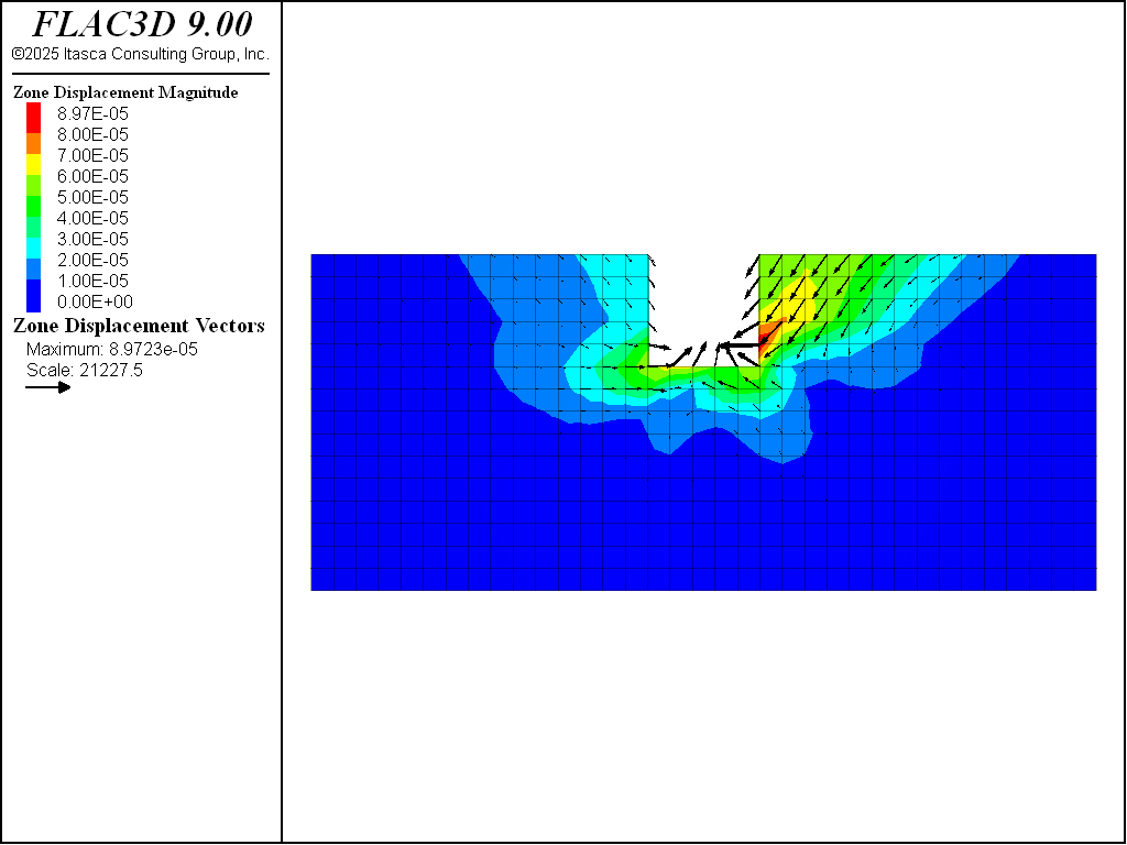
Figure 5: Displacement vectors from creep loading at end of simulation, case \(\theta = 30^{\circ}\).

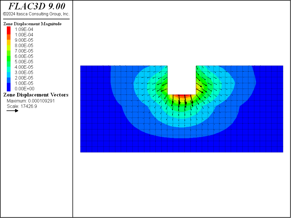
Figure 6: Displacement vectors from static loading from standing water, case \(\theta = 45^{\circ}\).

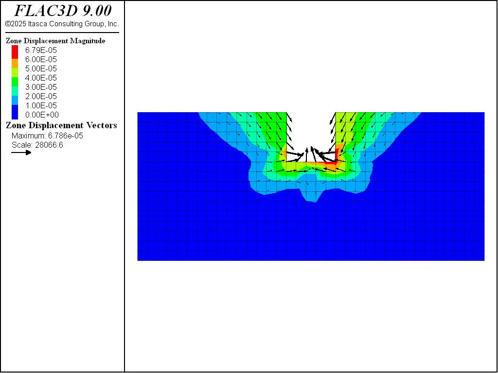
Figure 7: Displacement vectors from creep loading at end of simulation, case \(\theta = 45^{\circ}\).

The overall trend of creep displacements observed on the river banks for the 60 degree case (see Figure 9) is the reverse of the trend predicted for the 30 degree case (see Figure 5).

Figure 8: Displacement vectors from static loading from standing water, case \(\theta = 60^{\circ}\).

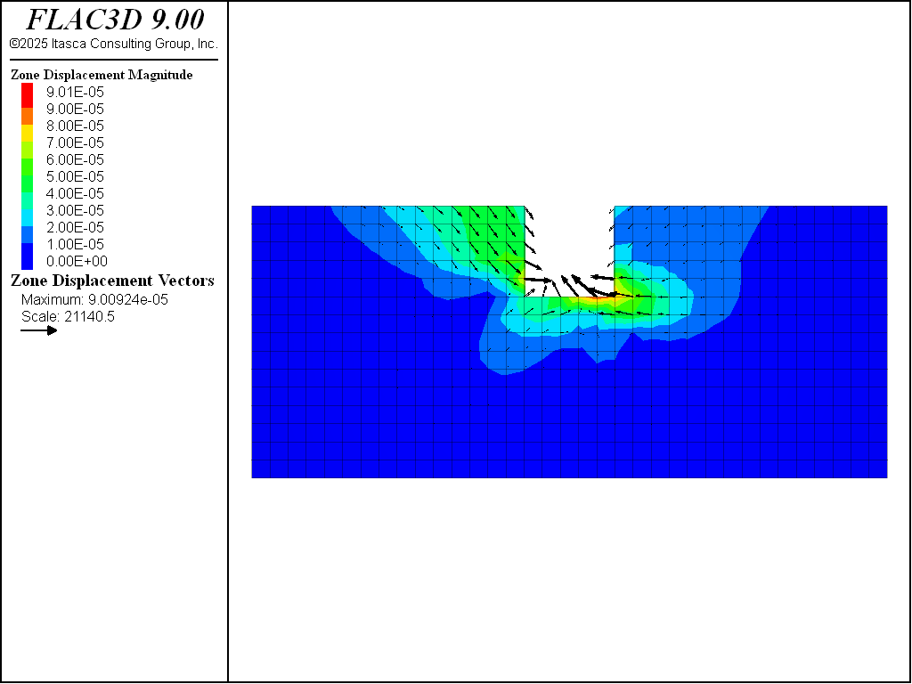
Figure 9: Displacement vectors from creep loading at end of simulation, case \(\theta = 60^{\circ}\).

It appears that both direct and complementary shearing modes are represented in the simulation results obtained for the cases investigated (see Figure 11).

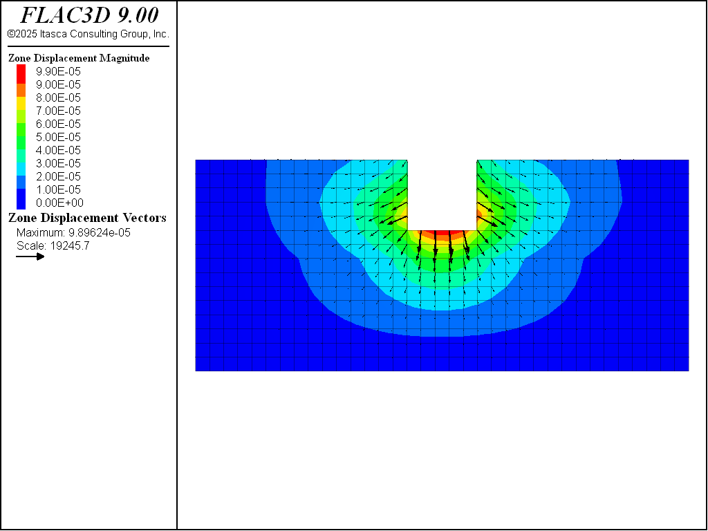
Figure 10: Displacement vectors from static loading from standing water, case \(\theta = 75^{\circ}\).

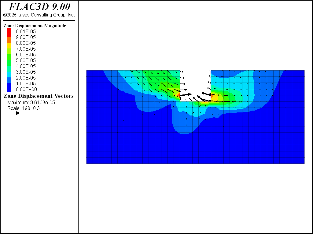
Figure 11: Displacement vectors from creep loading at end of simulation, case \(\theta = 75^{\circ}\).

The creep displacements induced by the shear stresses (caused by valley excavation and mechanical loading from the standing water) along the vertical joint plane in the COMBA layer are symmetric in this case (see Figure 12 and Figure 13), as expected.

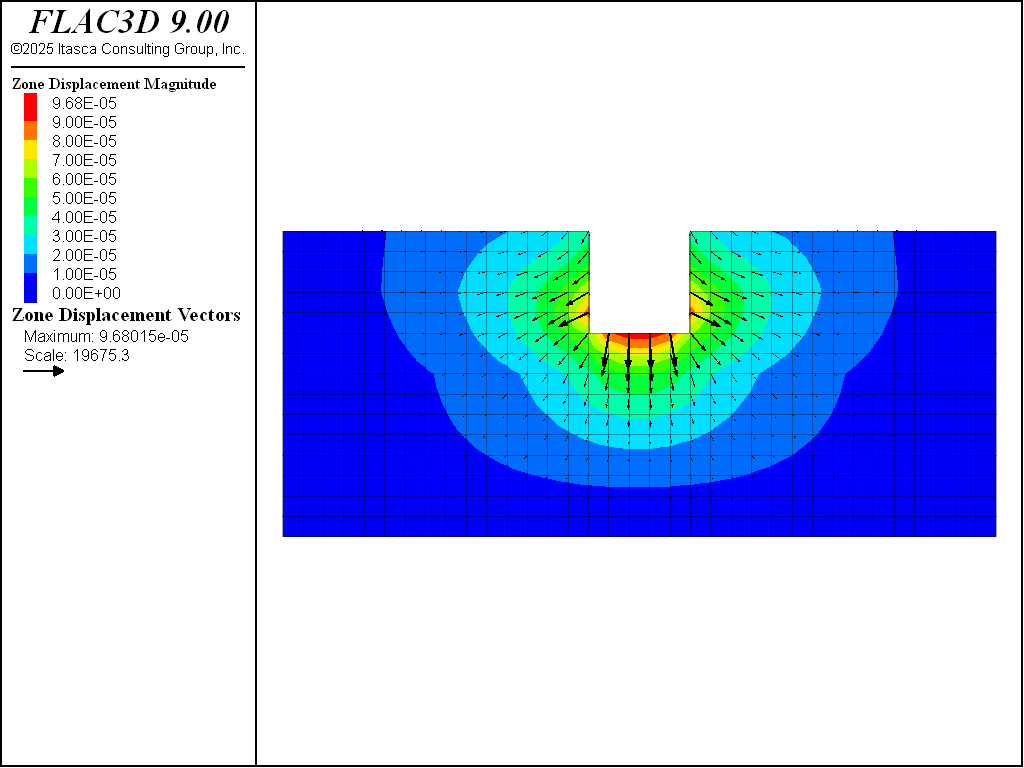
Figure 12: Displacement vectors from static loading from standing water, case \(\theta = 90^{\circ}\).

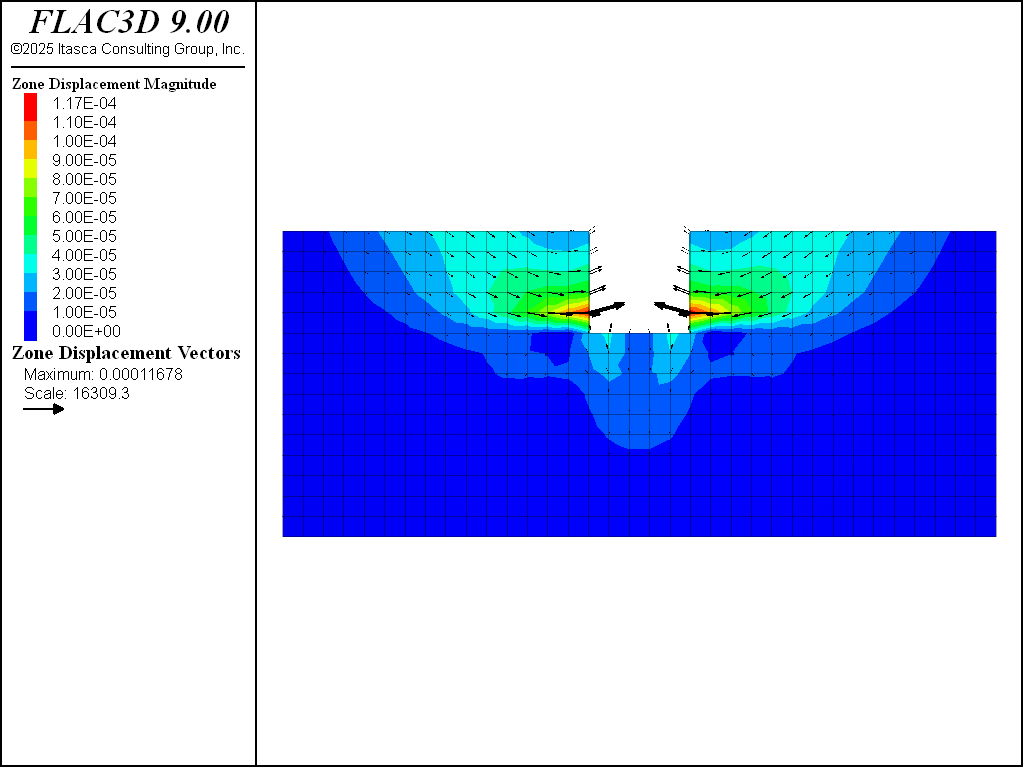
Figure 13: Displacement vectors from creep loading at end of simulation, case \(\theta = 90^{\circ}\).

Displacement Histories

The horizontal displacement at different elevations on the left and right river banks are monitored during the creep simulations. The location of the monitoring points is shown in Figure 14.

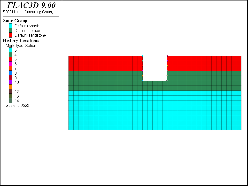
Figure 14: History locations of monitoring points.

The horizontal displacement at the monitoring points versus creep time is plotted through Figure 15 to Figure 20. The plots show a relatively sharp increase in horizontal displacement at the start of the simulation, and an evolution towards a steady-state of deformation by the end of the runs.

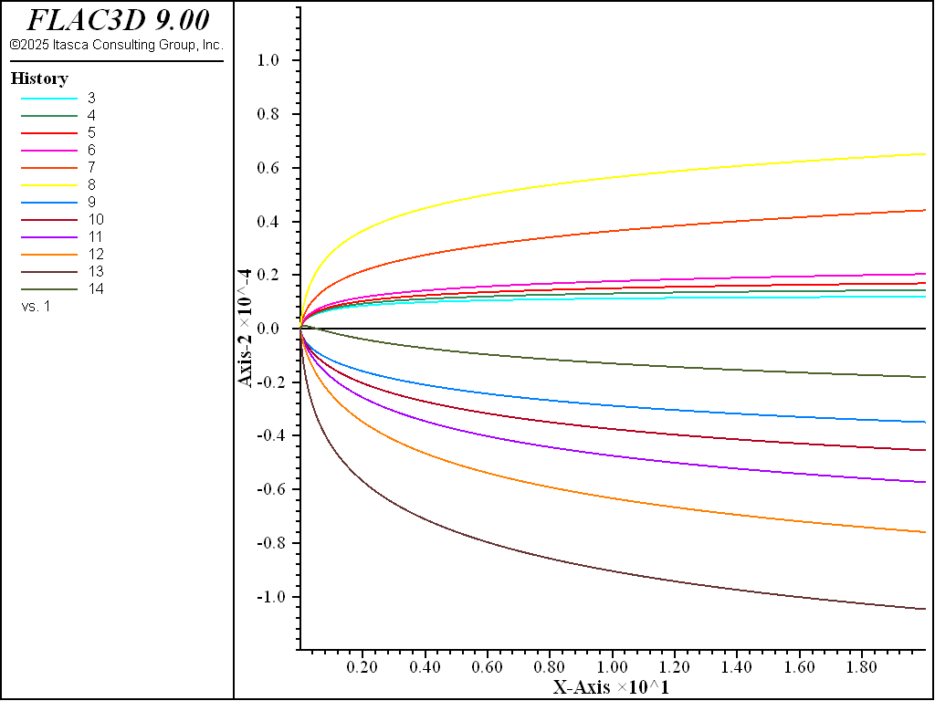
Figure 15: Horizontal displacement versus creep time at monitoring points, case \(\theta = 15^{\circ}\).

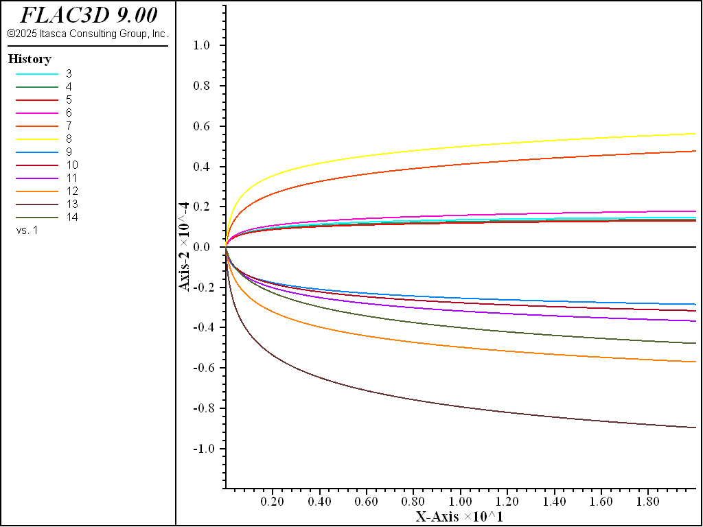
Figure 16: Horizontal displacement versus creep time at monitoring points, case \(\theta = 30^{\circ}\).

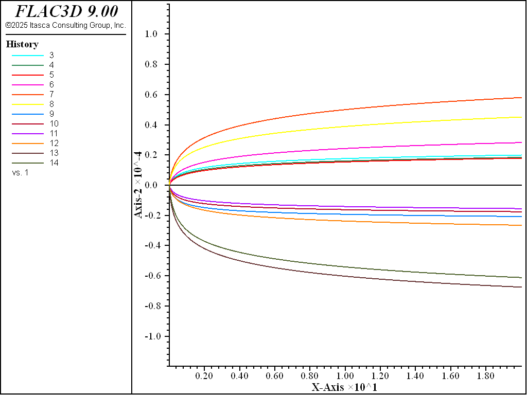
Figure 17: Horizontal displacement versus creep time at monitoring points, case \(\theta = 45^{\circ}\).

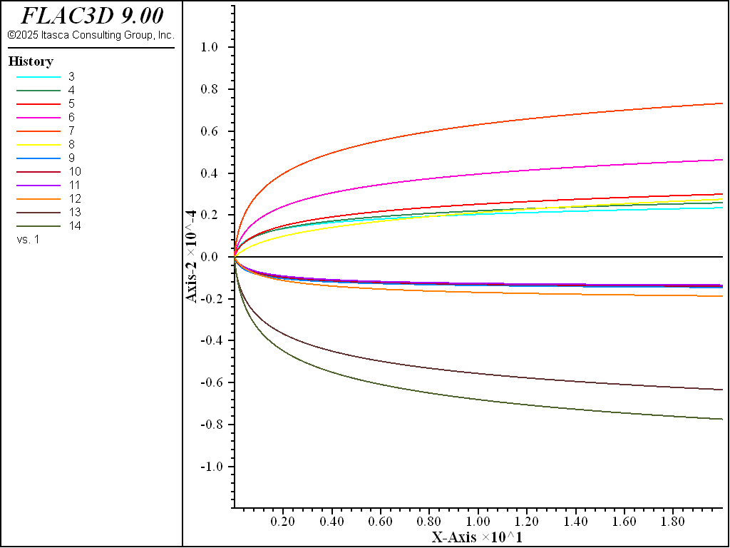
Figure 18: Horizontal displacement versus creep time at monitoring points, case \(\theta = 60^{\circ}\).

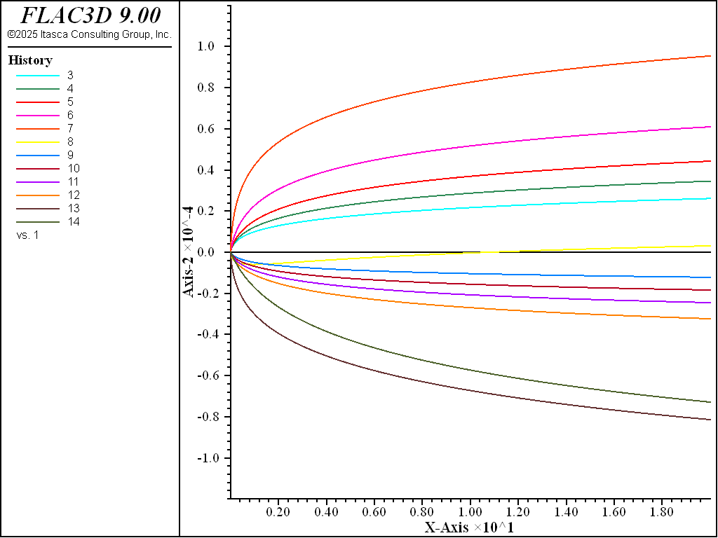
Figure 19: Horizontal displacement versus creep time at monitoring points, case \(\theta = 75^{\circ}\).

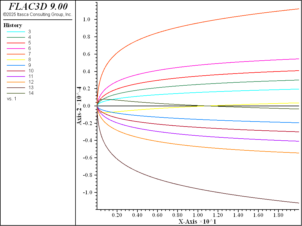
Figure 20: Horizontal displacement versus creep time at monitoring points, case \(\theta = 90^{\circ}\).

break

Data Files

valleyCreepDeformation-dip15.dat

;----------------------------------
; Simple valley - Comba with creep
;----------------------------------
model new
model title 'Simple Valley - COMBA model with creep'
model large-strain off
fish automatic-create off
model configure creep
model gravity 10
;
zone create brick size 35 1 15
zone group 'sandstone' range position-z 12 15
zone group 'comba' range position-z 8 12
zone group 'basalt' range position-z 0 8
;
zone cmodel assign elastic
zone property density 1800 bulk 2e9 shear 1e9 
;
fish define setup
  global teta  =  15.
  local  alpha = (90. + teta)*math.degrad
  global nx_   = math.cos(alpha)
  global nz_   = math.sin(alpha)
end
[setup]
;
zone cmodel assign columnar-basalt range group 'comba'
zone property density 1500 young 1.35e9 poisson 0.35 range group 'comba'
zone property flag-matrix-plastic off space-1 1.0 range group 'comba'
zone property stiffness-normal-1 3e9 stiffness-shear-1 3e9 range group 'comba'
zone property creep-coefficient-1 0.002 creep-exponent-1 4 range group 'comba'
zone property joint-friction-1 30 joint-tension-1 1e10 range group 'comba'
zone property normal-x-1 [nx_] normal-y-1 0.0 normal-z-1 [nz_] range group 'comba'
;
zone gridpoint fix velocity-x 0 range position-x 0
zone gridpoint fix velocity-x 0 range position-x 35
zone gridpoint fix velocity-y 0 
zone gridpoint fix velocity 0 0 0 range position-z 0
; --- set strength high ---
zone property joint-cohesion-1 1e20 range group 'comba'
;
model creep active off
model solve convergence 0.01
;
fish operator iso_stress(p_z)
    zone.stress.xx(p_z) = zone.stress.zz(p_z)
    zone.stress.yy(p_z) = zone.stress.zz(p_z)
end
[iso_stress(::zone.list)]
model solve convergence 0.01
;
zone gridpoint initialize displacement 0 0 0
zone cmodel assign null range position-x 15 20 position-z 10 15
model solve convergence 0.01
model save 'ini'
; --- water load ---
zone gridpoint initialize displacement 0 0 0
zone face apply stress-normal -14e4 gradient 0 0 1e4 ...
    range position-x 14.9 20.1 position-z 9.9 14.1
model solve convergence 0.01
; --- reset strength to realistic value ---
zone property joint-cohesion-1 0. range group 'comba'
model solve convergence 0.01
model save 'loaded-dip15'
;
zone gridpoint initialize displacement 0 0 0
zone gridpoint initialize velocity 0 0 0
;
model creep active on
model history creep time-total
model history mechanical unbalanced-maximum
zone history displacement-x position 15 0 15
zone history displacement-x position 15 0 14
zone history displacement-x position 15 0 13
zone history displacement-x position 15 0 12
zone history displacement-x position 15 0 11
zone history displacement-x position 15 0 10
zone history displacement-x position 20 0 15
zone history displacement-x position 20 0 14
zone history displacement-x position 20 0 13
zone history displacement-x position 20 0 12
zone history displacement-x position 20 0 11
zone history displacement-x position 20 0 10
;
model creep timestep automatic
model creep timestep starting 1e-8
model creep timestep minimum 1e-8
model creep timestep maximum 1e-3
model solve creep time-total 20
model save "valley-dip15"
;