Steady-State Fluid Flow Using Simple-Fluid Option
Note
The project file for this example is available to be viewed/run in FLAC3D. The project’s main data files are shown at the end of this example.
This example is the classical problem of steady-state seepage flow through a homogeneous embankment with vertical slopes exposed to different water levels and resting on an impermeable base. The total discharge, \(Q\), and the length of seepage face, \(s\), are compared to the exact solutions. Figure 1 shows the geometry and boundary conditions of the problem. This example has been solved in Steady-State Fluid Flow with a Free Surface. Here it is solved using the simple-fluid logic, with both explicit and implicit algorithms.
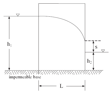
Figure 1: Problem geometry and boundary conditions.
The fluid is homogeneous, flow is governed by Darcy’s law, and it is assumed that the pores of the soil beneath the phreatic surface are completely filled with water and the pores above it are completely filled with air. The width of the dam is \(L\), the head and tail water elevations above the impervious base are \(h_{1}\) and \(h_{2}\), respectively.
The exact solution for the total discharge through a dam section of unit thickness was shown by Charny (Harr 1991) to be given by Dupuit’s formula:
where \(k\) is mobility coefficient, \(\rho _{w}\) is water density and \(g\) is gravity. The length, \(s\), of the seepage face (elevation of the free surface on the downstream face of the dam above \(h_{2}\)) was obtained by Polubarinova-Kochina (1962), and is given in Figure 2 as a function of the characteristic dimensions of the problem.
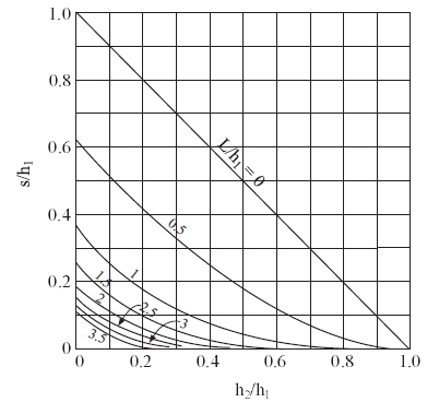
Figure 2: Seepage face solution after Polubarinova-Kochina (1962).
The FLAC3D simulation is conducted for a particular set of parameters:
L |
= |
9 m |
h1 |
= |
6 m |
h2 |
= |
1.2 m |
Several material properties are used:
hydraulic conductivity (\(k_h\)) |
10-6 (m/sec) |
porosity (\(n\)) |
0.3 |
water density (\(\rho_w\)) |
1000 kg/m3 |
water bulk modulus (\(K_f\)) |
1000 Pa |
soil dry density (\(\rho\)) |
2000 kg/m3 |
gravity (\(g\)) |
10 m/sec2 |
To use the simple-fluid logic, the command
model simple-saturation on
is used to activate the logic, which requires the fluid being configured and active in advance.
The Brooks-Corney relationship of apparent saturation and matrix suction with air-entry suction of 70 kPa and pore size index of 1.5 are used. The s-shape relationship of permeability ratio and apparent saturation is used so the specific discharge above phreatic surface is reasonably reduced. These two inputs are:
zone fluid saturation-suction brooks-corey 70 1.6
zone fluid permeability-saturation s-shape
Two cases corresponding to two different initial conditions can be used:
CASE 1: |
The water level in the embankment is initially at \(h\) = \(h_2\) = 1.2 m. The upstream level is raised to \(h\) = \(h_1\). |
CASE 2: |
The water level is initially at \(h\) = \(h_1\) = 6 m. The downstream level is lowered to \(h\) = \(h_2\). |
For Case 1, the command to set the initial conditions is
zone gridpoint initialize head 1.2 range position-z 0 1.2
For Case 2, the command to set the initial conditions is
zone gridpoint initialize head 6 range position-z 0 6
It shows that both cases have identical results, either for explicit or implicit algorithm. Here only Case 1 is illustrated. the boundary conditions are
zone face apply head 6.0 range position-x 0.0
zone face apply head 1.2 range position-x 9.0 position-z 0.0 1.2
zone face apply pore-pressure 0.0 range position-x 9.0 position-z 1.2 1.8
Note that, applying head conditions does not need to use the gradient which is required as applying pore-pressure conditions in Steady-State Fluid Flow with a Free Surface.
Figure 3 plots pore-pressure contour. Figure 3 plots apparent saturation distribution. Figure 3 plots permeability ratio distribution. Figure 3 plots head contour. Figure 3 through Figure 6 present the results using the explicit algorithm and all plot phreatic surface which is calculated/visualized at zero pore-pressure contour or iso-surface.
break

Figure 3: Steady-state flow vectors and pore-pressure distributions with explicit algorithm.

Figure 4: Steady-state flow vectors and head distributions with explicit algorithm.

Figure 5: Steady-state flow vectors and apparent saturation distributions with explicit algorithm.

Figure 6: Steady-state flow vectors and apparent saturation distributions with explicit algorithm.
For comparison, Figure 7 through Figure 10 present the corresponding results using the implicit algorithm. It is observed that the results are close between explicit and implicit algorithms. However, the fluid time step using implicit algorithm is 1000 while it is only 5.4 if using explicit algorithm. The benefit of quicker calculation with implicit algorithm is impossible if not using the simple-fluid logic.

Figure 7: Steady-state flow vectors and pore-pressure distributions with implicit algorithm.

Figure 8: Steady-state flow vectors and head distributions with implicit algorithm.

Figure 9: Steady-state flow vectors and apparent saturation distributions with implicit algorithm.

Figure 10: Steady-state flow vectors and apparent saturation distributions with implicit algorithm.
Reference
Harr, M. E. Groundwater and Seepage. Dover (1991).
Data Files
FreeSurfaceSimpleFluid.dat
model new
model title "Steady state flow through a vertical embankment - simple-fluid"
;
model large-strain off
program call 'fishFunctions'
model configure fluid
model fluid active on
model simple-saturation on
model mechanical active off
model gravity 0 0 -10

zone create brick size 60 1 40 point 1 (9.0,0,0) point 2 (0,0.15,0) ...
                               point 3 (0,0,6.0)
; --- fluid flow model ---
zone fluid cmodel assign isotropic
zone fluid property hydraulic-conductivity 1e-6 porosity 0.3
zone fluid saturation-suction brooks-corey 70 1.6
zone fluid permeability-saturation s-shape
;
zone initialize fluid-density 1e3
zone gridpoint initialize fluid-modulus 2e6
zone gridpoint initialize saturation 1.0
;case 1
zone gridpoint initialize head 1.2 range position-z 0.0 1.2
;case 2
;zone gridpoint initialize head 6 range position-z 0.0 6.0
;
zone face apply head 6.0 range position-x 0.0
zone face apply head 1.2 range position-x 9.0 position-z 0.0 1.2
zone face apply pore-pressure 0.0 range position-x 9.0 position-z 1.2 1.8
; --- test ---
model solve ratio-flow 1.e-3
;
[show_seepage_face]
fish list [qflac] [qsol]
;
model save 'freeSurface'
FreeSurfaceSimpleFluid-implicit.dat
model new
model title "Steady state flow through a vertical embankment - simple-fluid"
;
model large-strain off
program call 'fishFunctions'
model configure fluid
model fluid active on
model simple-saturation on
model mechanical active off
model gravity 0 0 -10

zone create brick size 60 1 40 point 1 (9.0,0,0) point 2 (0,0.15,0) ...
                               point 3 (0,0,6.0)
; --- fluid flow model ---
zone fluid cmodel assign isotropic
zone fluid property hydraulic-conductivity 1e-6 porosity 0.3
zone fluid saturation-suction brooks-corey 70 1.6
zone fluid permeability-saturation s-shape
;
zone initialize fluid-density 1e3
zone gridpoint initialize fluid-modulus 2e6
zone gridpoint initialize saturation 1.0
;case 1
zone gridpoint initialize head 1.2 range position-z 0.0 1.2
;case 2
;zone gridpoint initialize head 6 range position-z 0.0 6.0
;
zone face apply head 6.0 range position-x 0.0
zone face apply head 1.2 range position-x 9.0 position-z 0.0 1.2
zone face apply pore-pressure 0.0 range position-x 9.0 position-z 1.2 1.8
;
model step 100 ; always do few explicit steps first
zone fluid implicit on solver-jacob
model fluid timestep fix 1e3
;
model solve ratio-flow 1.e-3
;
[show_seepage_face]
fish list [qflac] [qsol]
;
model save 'freeSurface-implicit'
model new
model title "Steady state flow through a vertical embankment - simple-fluid"
;
model large-strain off
program call 'fishFunctions'
model configure fluid
model fluid active on
model simple-saturation on
model mechanical active off
model gravity 0 0 -10

zone create brick size 60 1 40 point 1 (9.0,0,0) point 2 (0,0.15,0) ...
                               point 3 (0,0,6.0)
; --- fluid flow model ---
zone fluid cmodel assign isotropic
zone fluid property hydraulic-conductivity 1e-6 porosity 0.3
zone fluid saturation-suction brooks-corey 70 1.6
zone fluid permeability-saturation s-shape
;
zone initialize fluid-density 1e3
zone gridpoint initialize fluid-modulus 2e6
zone gridpoint initialize saturation 1.0
;case 1
zone gridpoint initialize head 1.2 range position-z 0.0 1.2
;case 2
;zone gridpoint initialize head 6 range position-z 0.0 6.0
;
zone face apply head 6.0 range position-x 0.0
zone face apply head 1.2 range position-x 9.0 position-z 0.0 1.2
zone face apply pore-pressure 0.0 range position-x 9.0 position-z 1.2 1.8
; --- test ---
model solve ratio-flow 1.e-3
;
[show_seepage_face]
fish list [qflac] [qsol]
;
model save 'freeSurface'
| Was this helpful? ... | Itasca Software © 2024, Itasca | Updated: Nov 12, 2025 |
