Lined Circular Tunnel in an Elastic Medium with Anisotropic Stresses

Problem Statement

Note

To view this project in FLAC3D, use the menu command Help ‣ Examples…. Choose “Structure/Liner/LinedCircularTunnel” and select “LinedCircularTunnel.prj” to load. The main data file used is shown at the end of this example. The remaining data files can be found in the project.

A circular tunnel with a radius of 5 m is located at 30 m depth in a soft elastic soil. The in-situ stresses are 600 kPa vertical and 300 kPa horizontal. The tunnel is supported by a 125 mm thick shotcrete liner. The support is installed simultaneously with the excavation in a preexisting anisotropic biaxial stress field. The support displacements and stress resultants (in terms of thrust and moment), and the interface contact stresses are computed under plane-strain conditions for the two limiting conditions of no-slip (no relative shear displacement) and full-slip (no shear stress transmission) at the ground-support interface. These computed values are compared with the analytical solution of Einstein and Schwartz (1979).

Analytical Solution

The analytical solution (Einstein and Schwartz 1979) is expressed using the notation in Figure 1. The support displacements consist of a radial, \(u_s\), and a tangential, \(v_s\), component. The internal stresses consist of a circumferential thrust, \(T\), and a bending moment, \(M\). The interface contact stresses consist of a normal, \(\sigma_R\), and a shear, \(\tau_{R\theta}\), component.

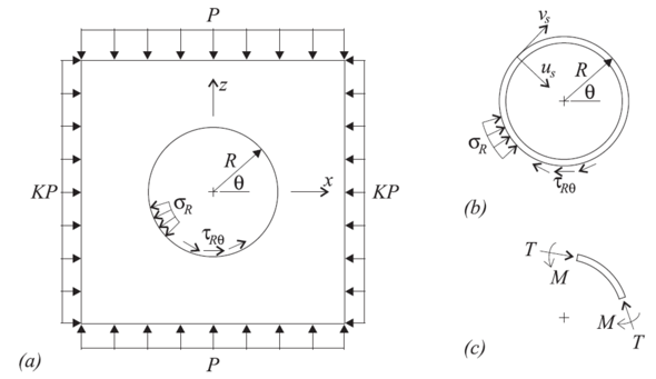
Figure 1: Notation for analytical solution: (a) ground medium; (b) tunnel liner; and (c) positive sense of internal stress resultants in liner.

No-Slip Solution — For the no-slip solution, the interface boundary condition consists of no relative shear displacement between the ground and the support. The no-slip solution is given in the following equations:

\[\begin{split}\begin{split} u_s &= {PR(1 + \nu) \over E} \biggl\{ {1\over2}(1 + K)a^*_0 + {1\over2}(1 - K)\left[4(1 - \nu)b^*_2 - 2a^*_2 \right]\cos 2\theta \biggr\} \\ v_s &= {PR(1 + \nu) \over E} \biggl\{ -(1 - K)\left[a^*_2 + (1 - 2\nu) b^*_2 \right]\sin 2\theta \biggr\} \\ T &= {P R \over 2} \biggl\{ (1 + K)(1 - a^*_0) + (1 - K)\left[1 + 2a^*_2 \right]\cos 2\theta \biggr\} \\ M &= {P R^2 \over 2} \biggl\{ {1\over2}(1 - K)\left[1 - 2a^*_2 + 2b^*_2 \right]\cos 2\theta \biggr\} \\ \sigma_R &= {P \over 2} \biggl\{ (1 + K)(1 - a^*_0) - (1 - K)\left[1 - 6a^*_2 + 4b^*_2 \right]\cos 2\theta \biggr\} \\ \tau_{R\theta} &= {P \over 2} \biggl\{ (1 - K)\left[1 + 6a^*_2 - 2b^*_2 \right]\sin 2\theta \biggr\} \end{split}\end{split}\]

where:	\(\theta\)	=	angular location (counterclockwise with respect to horizontal);
	\(R\)	=	tunnel radius;
	\(P\)	=	vertical stress;
	\(K\)	=	ratio of horizontal-to-vertical stress;
	\(E\)	=	Young’s modulus of the ground mass;
	\(\nu\)	=	Poisson’s ratio of the ground mass; and
	\(a^*_0,a^*_2,b^*_2\)	=	dimensionless coefficients (see the next equations below).

\[\begin{split}\begin{split} a^*_0 &= { C^* F^* (1 - \nu) \over C^* + F^* + C^* F^* (1 - \nu)} \\ a^*_2 &= \beta b^*_2 \\ b^*_2 &= { C^* (1 - \nu) \over 2\bigl[C^* (1 - \nu) + 4\nu - 6\beta - 3\beta C^*(1 - \nu) \bigr]} \\ \beta &= { (6 + F^*) C^* (1 - \nu) + 2F^* \nu \over 3F^* + 3C^* + 2C^* F^* (1 - \nu)} \end{split}\end{split}\]

where:

\(C^*\), \(F^*\)

=

compressibility and flexibility ratios, respectively (see the next two equations).

(1)\[\begin{split}\begin{split} C^* &= { E R (1 - \nu_s^2) \over E_s A_s (1 - \nu^2)} \\ F^* &= { E R^3 (1 - \nu_s^2) \over E_s I_s (1 - \nu^2)} \end{split}\end{split}\]

where:	\(E_s\)	=	Young’s modulus of the support;
	\(\nu_s\)	=	Poisson’s ratio of the support;
	\(A_s\)	=	average cross-sectional area of support per unit length of tunnel
			(for support of constant thickness \(t\), \(A_s = t\)); and
	\(I_s\)	=	moment of inertia of support per unit length of tunnel
			(for support of constant thickness \(t\), \(I_s = t^3/12\)).

Full-Slip Solution — For the full-slip solution, the interface boundary condition consists of no shear stress transmission between the ground and the support. The full-slip solution is given in the following equations:

\[ \begin{align}\begin{aligned}\begin{split}\begin{split} u_s &= {PR(1 + \nu) \over E} \biggl\{ {1\over2}(1 + K)a^*_0 - (1 - K)\left[(5 - 6\nu)a^*_2 - (1 - \nu) \right]\cos 2\theta \biggr\} \\ v_s &= {PR(1 + \nu) \over E} \biggl\{ {1\over2}(1 - K)\left[(5 - 6\nu)a^*_2 - (1 - \nu) \right]\sin 2\theta \biggr\} \\ \\\end{split}\\\begin{split} T &= {P R \over 2} \biggl\{ (1 + K)(1 - a^*_0) + (1 + K)\left[1 - 2a^*_2 \right]\cos 2\theta \biggr\} \\ M &= {P R^2 \over 2} \biggl\{ (1 - K)\left[1 - 2a^*_2 \right]\cos 2\theta \biggr\} \\ \\\end{split}\\\begin{split} \sigma_R &= {P \over 2} \biggl\{ (1 + K)(1 - a^*_0) - (1 - K)\left[3 - 6a^*_2 \right]\cos 2\theta \biggr\} \\ \tau_{R\theta} &= 0 \end{split}\end{split}\end{aligned}\end{align} \]

where:	\(\theta\)	=	angular location (counterclockwise with respect to horizontal);
	\(R\)	=	tunnel radius;
	\(P\)	=	vertical stress;
	\(K\)	=	ratio of horizontal-to-vertical stress;
	\(E\)	=	Young’s modulus of the ground mass;
	\(\nu\)	=	Poisson’s ratio of the ground mass; and
	\(a^*_0\), \(a^*_2\)	=	dimensionless coefficients (see the next equations).

\[\begin{split}\begin{split} a^*_0 &= { C^* F^* (1 - \nu) \over C^* + F^* + C^* F^* (1 - \nu)} \\ a^*_2 &= { (F^* + 6)(1 - \nu) \over 2F^* (1 - \nu) + 6(5 - 6\nu)} \end{split}\end{split}\]

where:

\(C^*\), \(F^*\)

=

compressibility and flexibility ratios, respectively (see equation (1) above).

FLAC3D Model

The problem is described in terms of the following parameters from the analytical solution:

Geometry
tunnel radius (\(R\))	5 m
In-Situ Stresses
vertical stress (\(P\))	600 kPa
ratio of horizontal-to-vertical stress (\(K\))	0.5
(\(\sigma_{xx}=-300\) kPa; \(\sigma_{zz}=-600\) kPa)
Ground Mass Properties
Young’s modulus (\(E\))	48 MPa
Poisson’s ratio (\(\nu\))	0.34
(shear modulus = 17.91 MPa; bulk modulus = 50 MPa)
Liner Properties
Young’s modulus (\(E_s\))	25 GPa
Poisson’s ratio (\(\nu_s\))	0.15
thickness (\(t\))	125 mm

The FLAC3D model simulates a thin slice of a circular tunnel in an infinite elastic ground mass with a preexisting anisotropic biaxial stress field subjected to plane-strain conditions. The geometry of the FLAC3D model is shown in Figure 2. The far-field boundaries are placed at a distance of 20 times the tunnel radius to approximate infinite boundaries. The in-situ stresses are installed in all zones and also applied as loads acting on the far-field boundaries. Plane-strain conditions are enforced by including a thin slice of material in the \(y\)-direction and imposing symmetry boundary conditions on these two surfaces. Symmetry boundary conditions are also imposed on the planes at \(x=0\) and \(z=0\). For gridpoints, this requires maintaining zero displacement normal to the plane. For nodes, this requires maintaining zero displacement normal to the plane and zero rotation about two axes that lie in the plane. (The appropriate nodal conditions are imposed by realigning and then fixing the appropriate node-local systems, and also specifying the proper velocity-fixity conditions — see Lined Tunnel (with liner elements) for a description of the procedure.)

The FLAC3D grid contains a single layer of zones in the \(y\)-direction and is graded as one moves away from the tunnel (see Figure 3). The model resolution is 24 zones along the tunnel boundary. Liner structural elements with a crosshatch mesh pattern (see Liner-Reinforced Beam for reasons why this mesh pattern is chosen) are attached to the zone faces lying along the tunnel boundary (see Figure 4). The liner-zone interface stiffnesses (\(k_n\) and \(k_s\)) are chosen using the liner-stiffness equation, and increasing the value by a factor of 100 as suggested in the text following this equation. We will confirm below that the criterion of small interface deformation is met for our system.

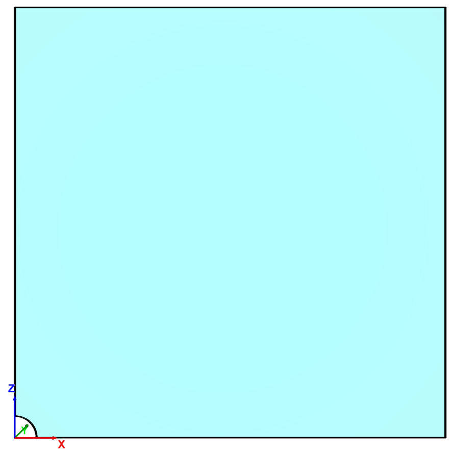
Figure 2: Geometry of the FLAC3D model.

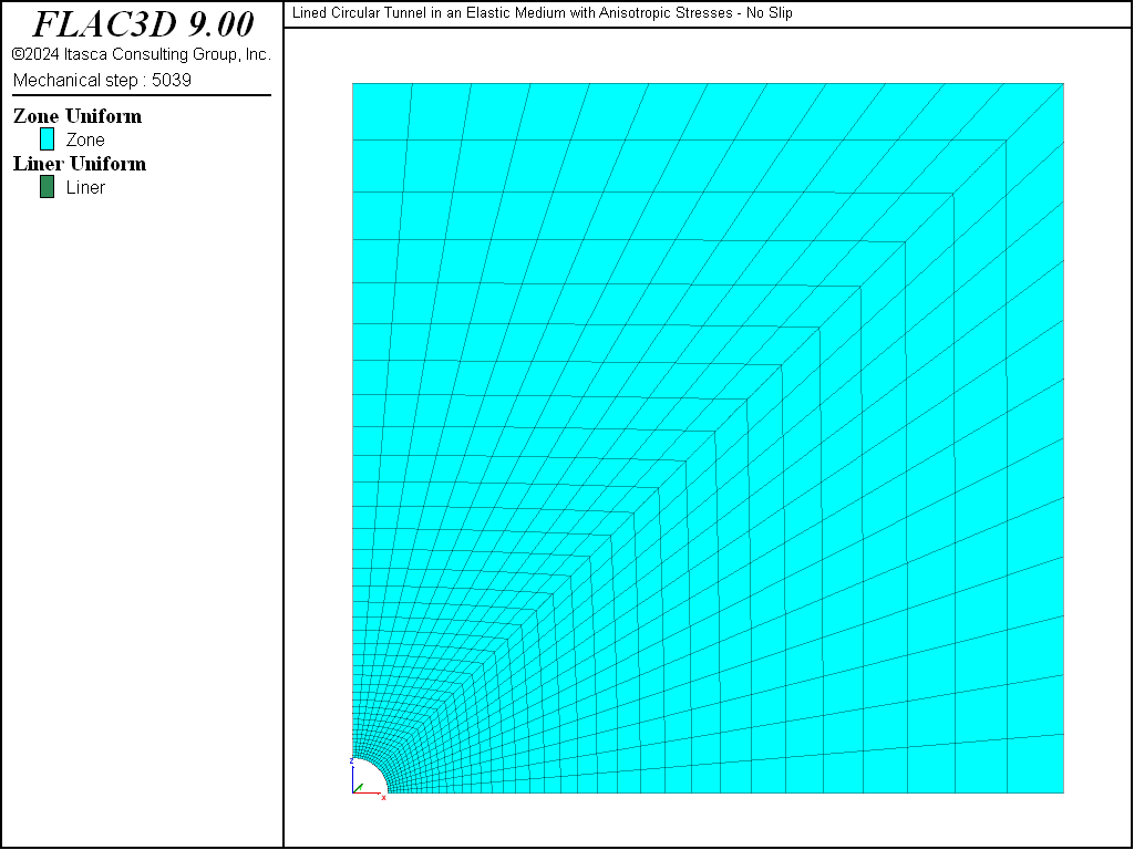
Figure 3: Zones in the FLAC3D model.

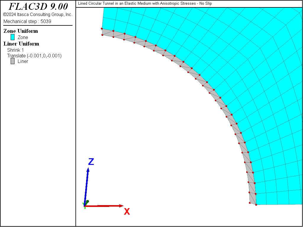
Figure 4: Liner elements, nodes, and zones in the FLAC3D model.

Results and Discussion — Qualitative Assessment

We confirm that the interface deformation is small relative to the zone deformation (and thus confirm that the elastic interface stiffnesses, \(k_n\) and \(k_s\), are large enough) by plotting the displacements of the gridpoints and nodes at the tunnel crown and springline (see Figure 5). The relative displacement between the gridpoints and nodes is small compared with the gridpoint displacement.

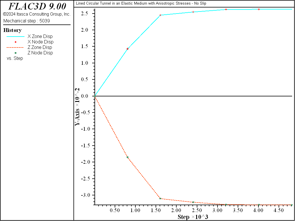
Figure 5: Displacements of gridpoints and nodes at tunnel crown and springline for no-slip case.

If the model is run with no support (by deleting the liner elements), the tunnel crown and springline both move inward (see Figure 6). When the support is included, the tunnel crown still moves inward, but the tunnel springline moves outward (see Figure 7), because the support resists the inward ground movement. If the liner is allowed to slip at the support-ground interface (by setting the liner property of coupling-cohesion-shear equal to zero), a relative shearing motion occurs between the liner and the ground (see Figure 8).

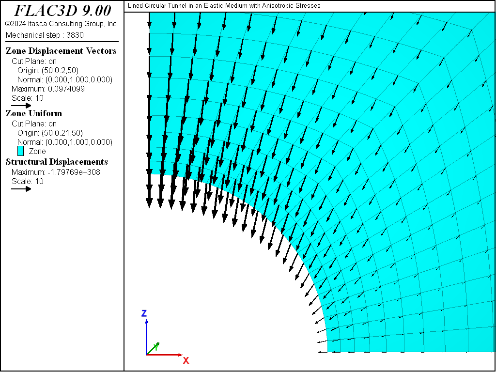
Figure 6: Displacement field of ground with no liner present.

Figure 7: Displacement field of liner and ground (no slip).

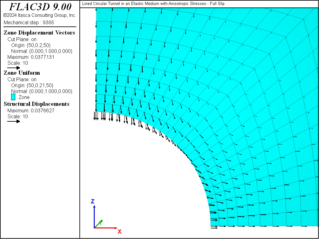
Figure 8: Displacement field of liner and ground (full slip).

The thrust, \(T\), and bending moment, \(M\), in the liner for both the no-slip and full-slip cases are shown in Figures #lined-noslip-thrustNy to 12. When the liner is allowed to slip, the thrust becomes more uniform and the bending moment increases slightly. We define a liner surface coordinate system whose \(x\)-axis lies along the tunnel axis (in the global \(y\)-direction), and whose \(z\)-axis is normal to the shell mid-surface (pointing inward). This corresponds to the surface = (0, 1, 0) direction during the stress recovery procedure. (The surface coordinate system needs to be defined — see Stress Recovery Procedure for details.) In terms of this system, the thrust corresponds with the membrane stress resultant, \(N_y\), where the \(y\)-direction lies along the tunnel circumference, and the bending moment corresponds with the bending stress resultant, \(M_y\). In these plots, the liner is oriented such that left-to-right corresponds with the angular location \(\theta\) in the closed-form solution varying from zero to ninety degrees. Note that these values of \(N_y\) and \(M_y\) are of opposite sign to the values of \(T\) and \(M\) from the analytical solution. (Positive \(N_y\) extends the shell, and positive \(M_y\) produces positive stress at the outer fiber on the side of the shell defined by the positive \(z\)-direction of the surface system.)

break

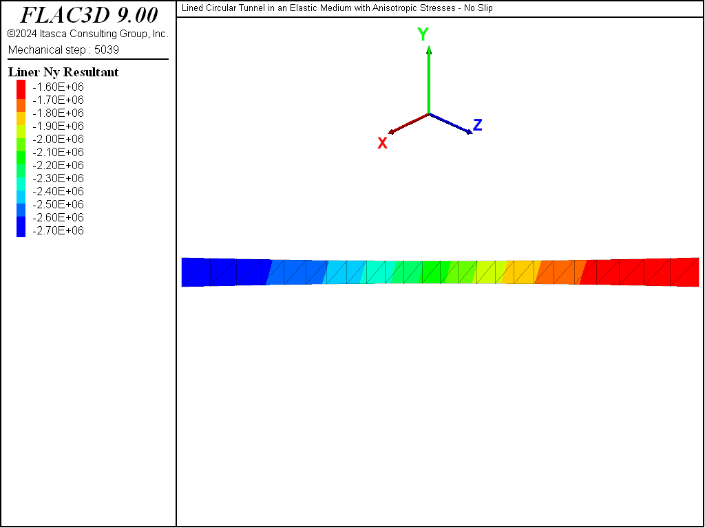
Figure 9: Thrust in liner (no slip).

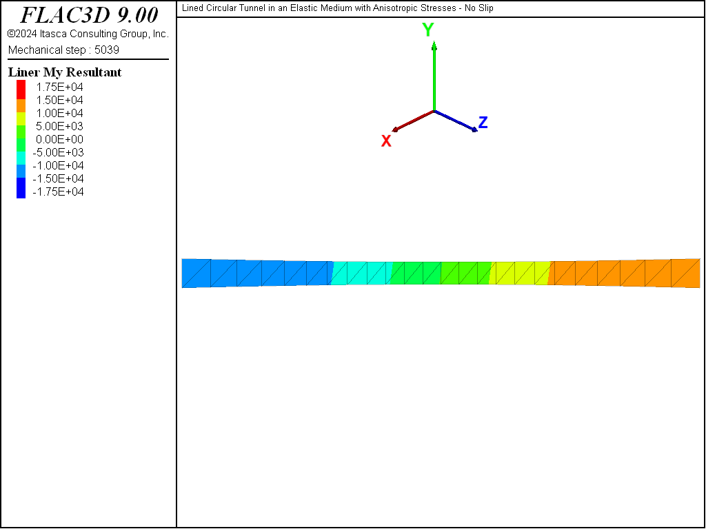
Figure 10: Bending moment in liner (no slip).

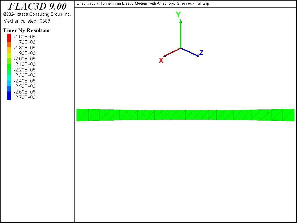
Figure 11: Thrust in liner (full slip).

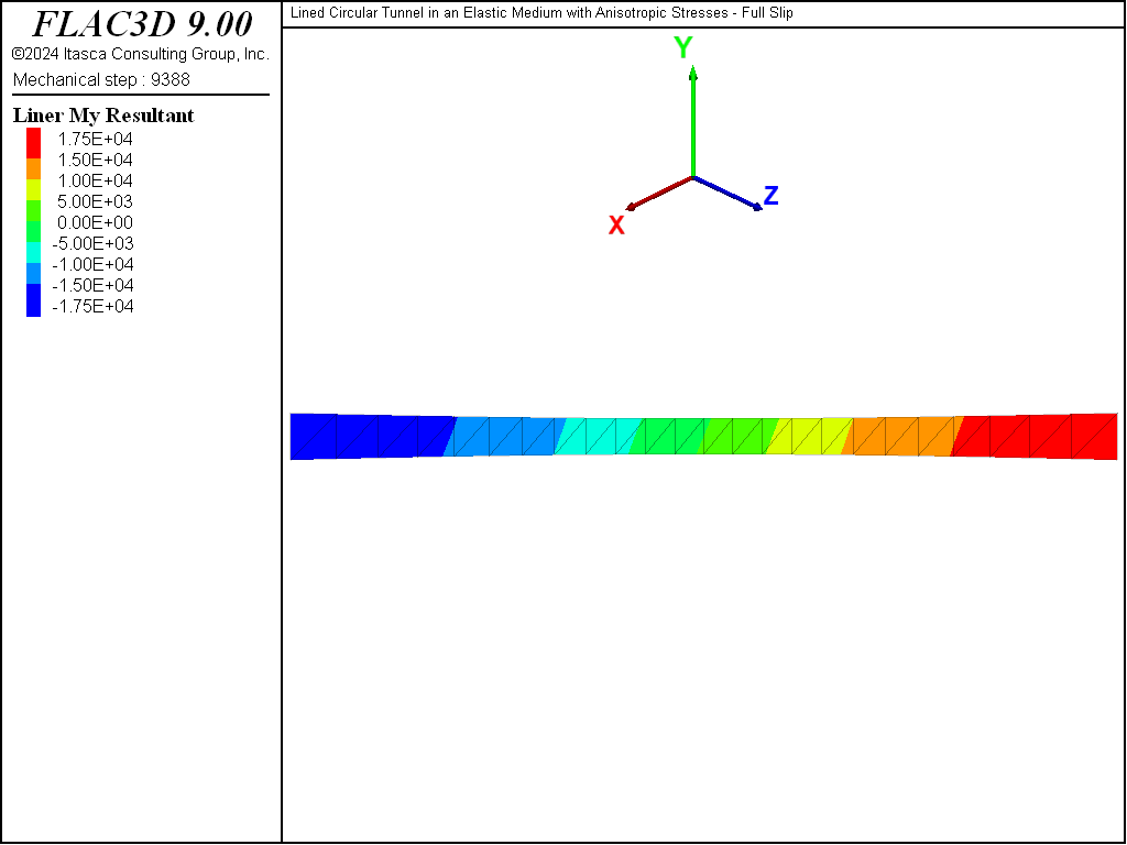
Figure 12: Bending moment in liner (full slip).

The interface contact stresses, \(\sigma_R\) and \(\tau_{R\theta}\), for both the no-slip and full-slip cases are shown in Figures 13 to 16. These values are obtained from the normal and shear coupling springs that join the liner nodes to the zones. Positive normal stresses indicate separation, and this convention is opposite to that of the analytical solution. The plotted shear stresses depict magnitude only; the direction can be printed or accessed by the FISH functions struct.liner.normal.dir and struct.liner.shear.dir.

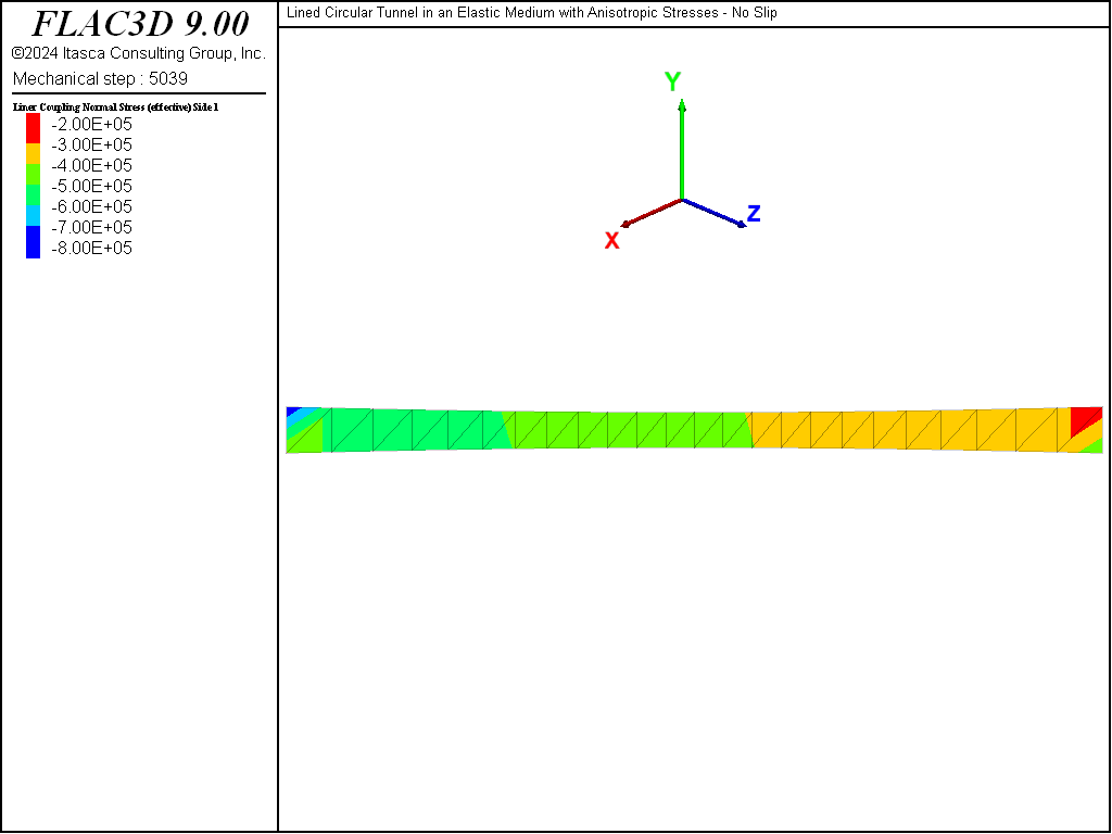
Figure 13: Interface normal contact stress (no slip).

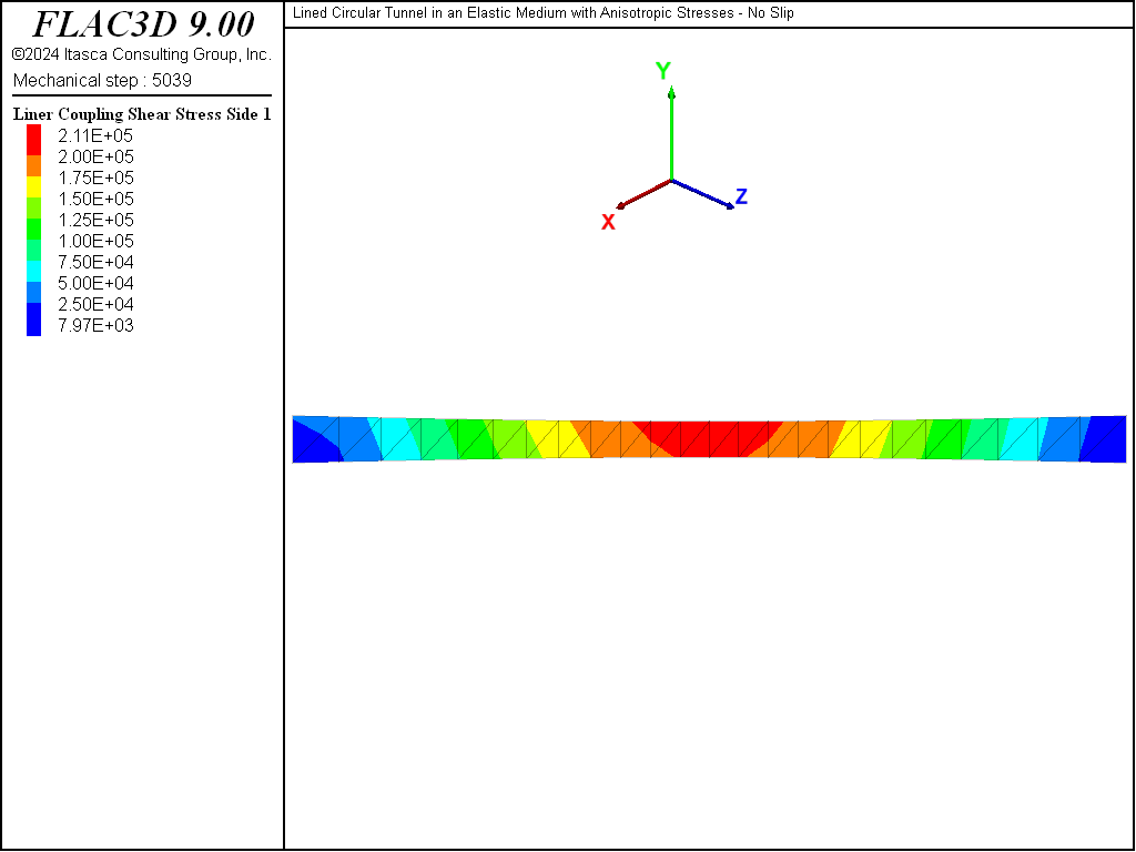
Figure 14: Interface shear contact stress (no slip).

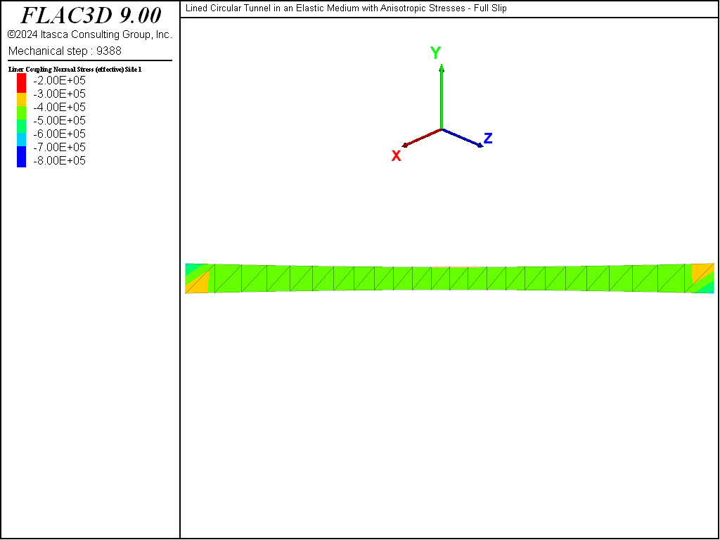
Figure 15: Interface normal contact stress (full slip).

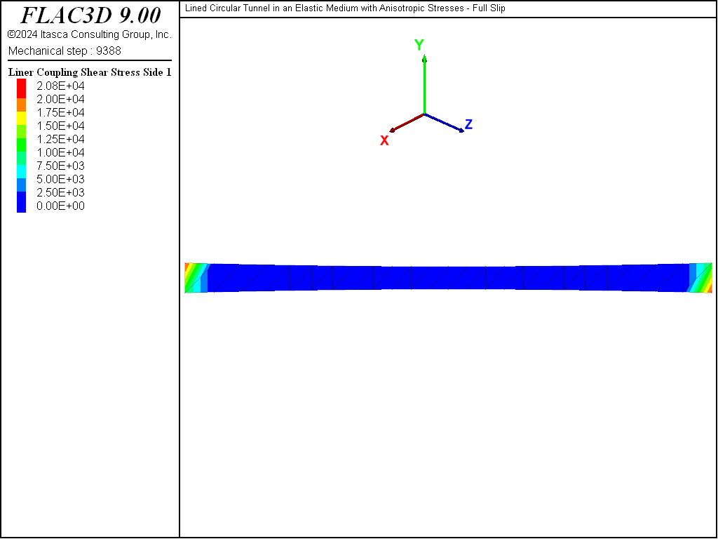
Figure 16: Interface shear contact stress (full slip).

Results and Discussion — Quantitative Assessment

A quantitative comparison of the support displacements, internal stresses, and interface contact stresses with the analytical solutions for both the no-slip and full-slip cases is provided in Figures 17 to 25. The FISH functions extract the necessary values from the FLAC3D model and compare them with the analytical values. Either the no-slip or full-slip analytical solution is used by setting the no_slip FISH variable to 1 or 0, respectively. The support displacements (\(u_s\) and \(v_s\)) are sampled at the nodes using the struct.node.disp.global FISH function. The internal stresses (\(T\) and \(M\)) are sampled at the element centroids using the struct.shell.resultant function. Also, the interface contact stresses (\(\sigma_R\) and \(\tau_{R\theta}\)) are sampled at the element centroids by computing the average value from the three coupling springs at the element nodes using the struct.liner.normal.stress and struct.liner.shear.stress functions.

For both the no-slip and full-slip cases, the responses compare well with the analytical solution. The support displacements match the analytical solution, with a maximum discrepancy of approximately 2% at the tunnel crown. The thrusts match the analytical solution, with a maximum discrepancy of approximately 1.2%. The interface contact stresses match the analytical solution away from the modeled ends (at \(\theta\) equals 0 and 90 degrees). There is an error of approximately 10% at the end locations (note the outliers in Figures 20 and 25) that arises from the lack of symmetry of the mesh. The area assigned to the two nodes at each end is not the same because it is the summation of one-third of the area of each element using the node. At each end, one node has twice the area of the other, and this affects the stress computation such that the result is nonsymmetric. Notice that the two outliers bound the analytical solution, and that their average value equals the analytical solution.

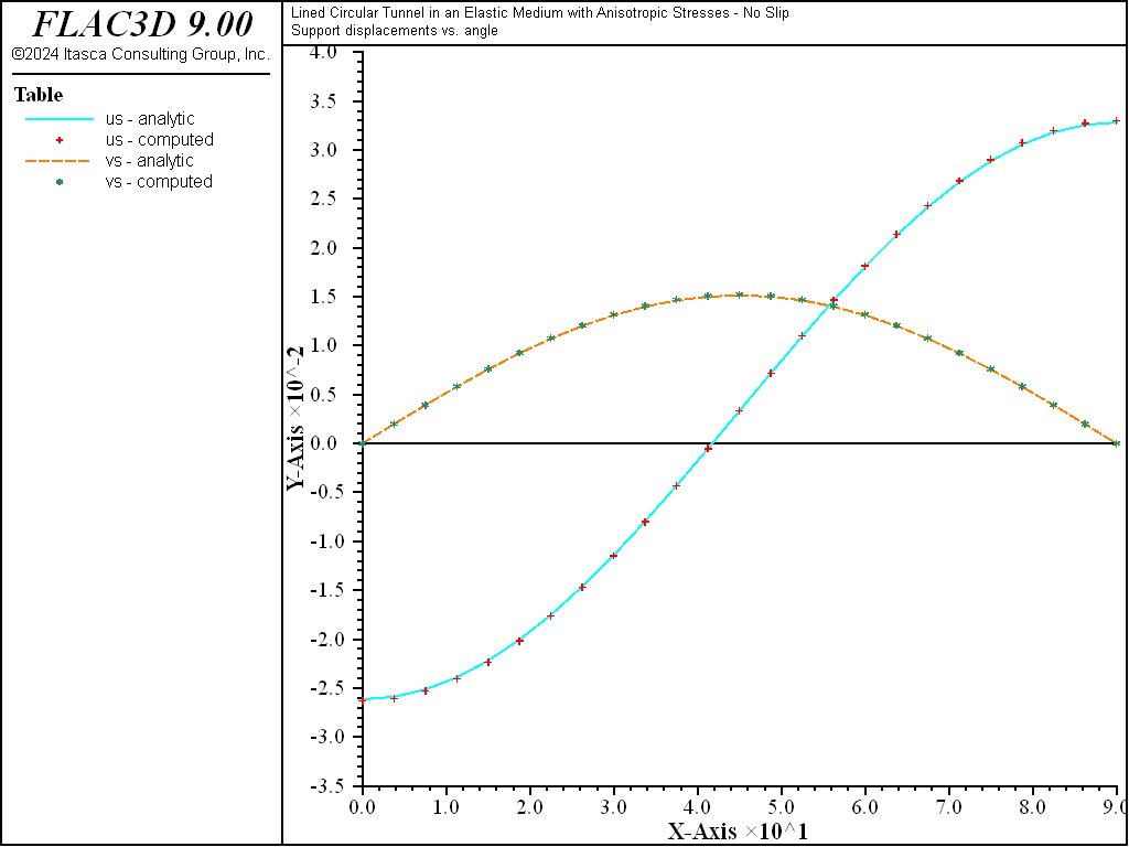
Figure 17: Radial and tangential support displacements versus angle (computed and analytical values, no slip).

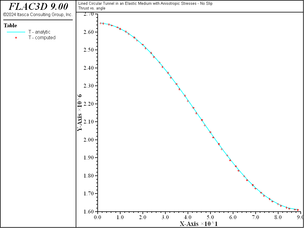
Figure 18: Thrust versus angle (computed and analytical values, no slip).

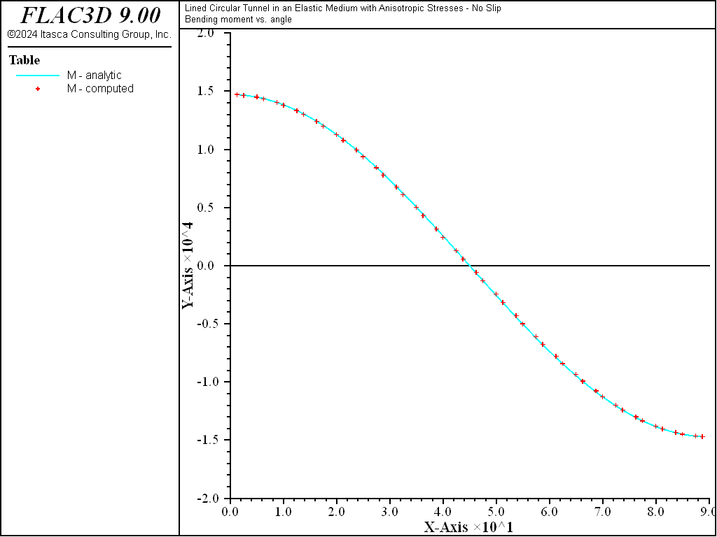
Figure 19: Bending moment versus angle (computed and analytical values, no slip).

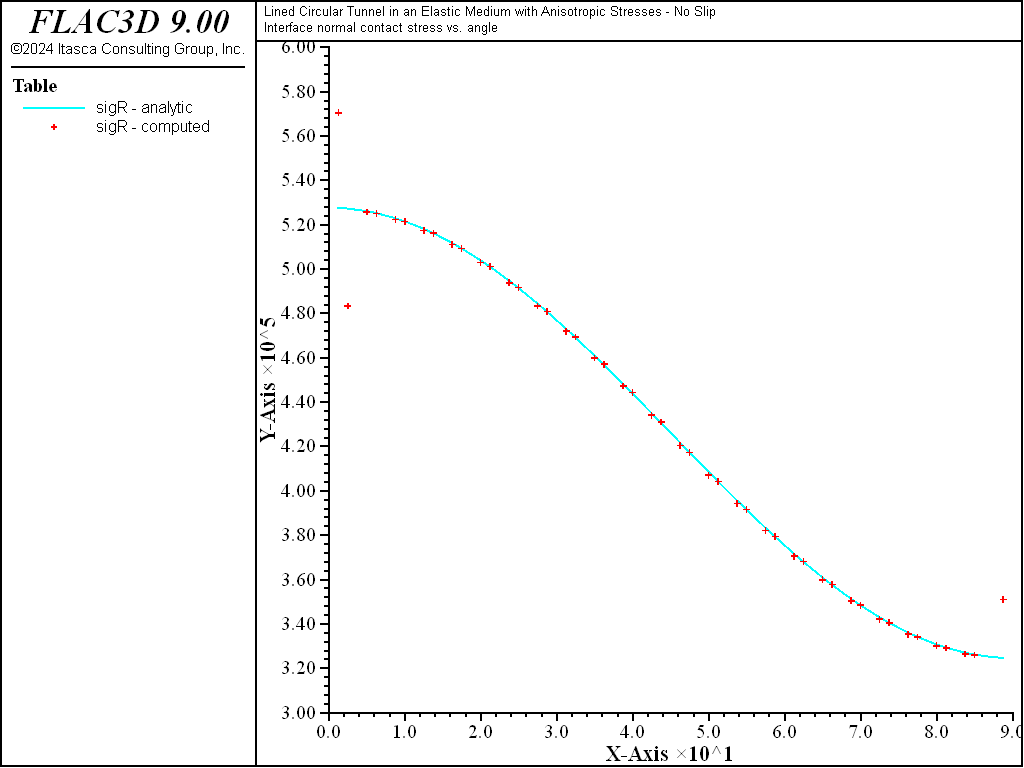
Figure 20: Interface normal contact stress versus angle (computed and analytical values, no slip).

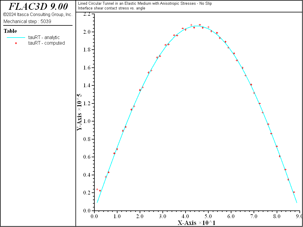
Figure 21: Interface shear contact stress versus angle (computed and analytical values, no slip).

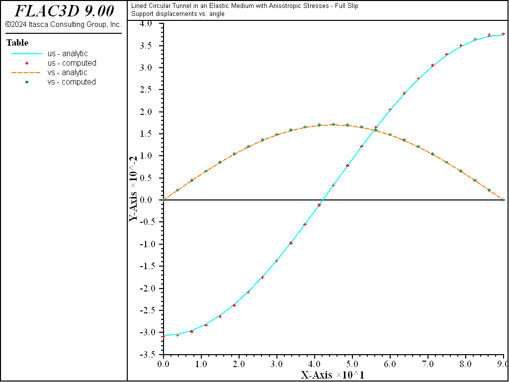
Figure 22: Radial and tangential support displacements versus angle (computed and analytical values, full slip).

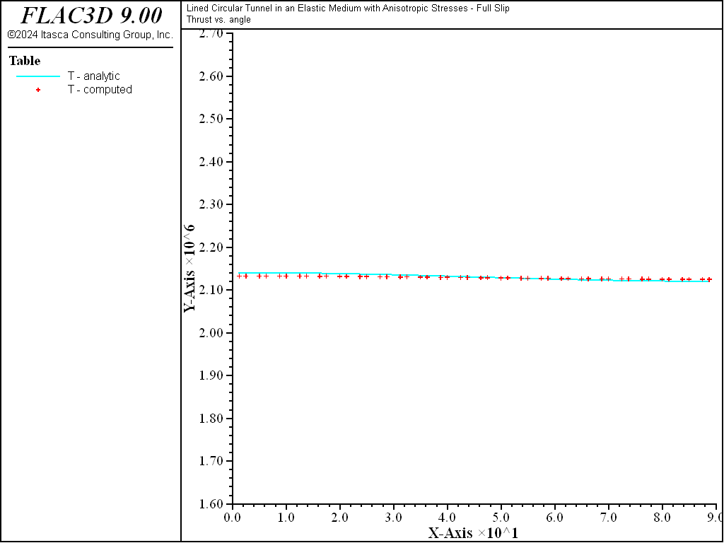
Figure 23: Thrust versus angle (computed and analytical values, full slip).

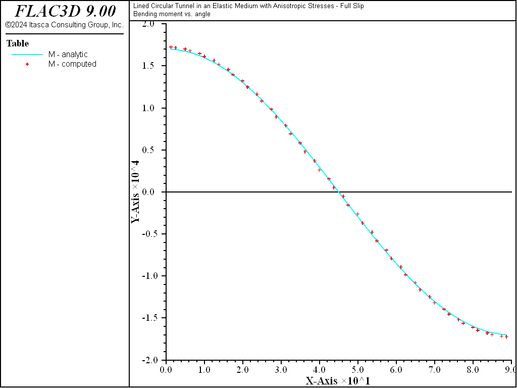
Figure 24: Bending moment versus angle (computed and analytical values, full slip).

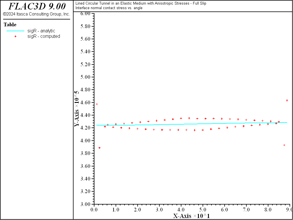
Figure 25: Interface normal contact stress versus angle (computed and analytical values, full slip).

Reference

Einstein, H. H., and C. W. Schwartz. “Simplified Analysis for Tunnel Supports,” J. Geotech. Engr. Div., 105(GT4): 499-518 (1979).

break

Data File

LinedCircularTunnel.dat

model new
model large-strain off
fish automatic-create off
[global t = 'Lined Circular Tunnel in an Elastic Medium']
[t += ' with Anisotropic Stresses']
model title [t]
; Create the ground mass (zones).
zone create radial-cylinder size 1 1 24 38 ratio 1 1 1 1.087 ...
                            point 1 (100,0,0) point 2 (0,0.4,0) ...
                            point 3 (0,0,100) dimension 5 5 5 5
; Material model and properties
zone cmodel assign elastic
zone property bulk 5e7 shear 1.791e7
; Name the model boundaries
zone face skin
; Create the support (linerSELs).
structure liner create by-zone-face range group 'West1'
structure liner cmodel assign elastic
structure liner property young 2.5e10 poisson 0.15 thickness 0.125 ...
                      coupling-stiffness-normal 2.0763e10 ...
                      coupling-stiffness-shear 2.0763e10 ...
                      coupling-cohesion-shear 1e20
; Install in-situ stresses in entire grid.
zone initialize stress xx -3e5 yy -3e5 zz -6e5
; Specify boundary conditions.
  ; Apply stresses at far-field boundaries
zone face apply stress-normal -3e5 range group 'East'
zone face apply stress-normal -6e5 range group 'Top'
  ; For the grid points (symmetry conditions)
zone face apply velocity-normal 0.0 range group 'West2' or 'Bottom'
zone face apply velocity-normal 0.0 range group 'North' or 'South'
  ; For the nodes (symmetry conditions)
structure node system-local x (1,0,0) y (0,-1,0)    ...
            range position-x 0   ; x=0 plane
structure node fix system-local                     ...
            range position-x 0
structure node fix velocity-x rotation-y rotation-z ...
            range position-x 0
structure node system-local x (0,0,-1) y (0,-1,0)   ...
            range position-z 0   ; z=0 plane
structure node fix system-local                     ...
            range position-z 0
structure node fix velocity-x rotation-y rotation-z ...
            range position-z 0
structure node fix velocity-y rotation-x rotation-z ...
            range position-y 0   ; y=0 plane
structure node fix velocity-y rotation-x rotation-z ...
            range position-y 0.4 ; y=Ymax plane
; Histories
model history mechanical ratio-local
zone history displacement-x position (5,0,0)        ; tunnel spring-line
zone history velocity-x     position (5,0,0)
structure node history displacement-x position (5,0,0)
structure node history velocity-x     position (5,0,0)
zone history displacement-z position (0,0,5)        ; tunnel crown
zone history velocity-z     position (0,0,5)
structure node history displacement-z position (0,0,5)
structure node history velocity-z     position (0,0,5)
history interval 10
;
model save 'starting'
; No support case
structure liner delete
model solve convergence 0.1
model title [t]
model save 'No Support'
; Slip case
model restore 'starting'
structure liner property coupling-cohesion-shear 0
model solve convergence 0.1
structure liner recover surface 0 1 0
structure liner recover resultants
model title [t + " - Full Slip"]
model save 'Full Slip'
; No slip case
model restore 'starting'
model solve convergence 0.1
structure liner recover surface 0 1 0
structure liner recover resultants
model title [t + " - No Slip"]
model save 'No Slip'