Massflow Parameter Study
Problem Statement
Note
To view these projects in MassFlow, use the menu command . Choose “MassFlow/ Examples/” and select a specific project for a specific example to load. The main data files used are shown at the end of this example. All data files are found in the projects.
The following examples are proposed to depict a simplified case of a caving mine modeled using MassFlow on gravity flow aspects of the operation. According to the block model, the ore is located only in the first 150 m above the footprint. Above that elevation, the rock mass is considered waste material (therefore inducing dilution). The base case considers the existence of an open-pit mine on the surface. A view of the initial geometry is presented in Figure Figure #massflow_ex1_fig1.
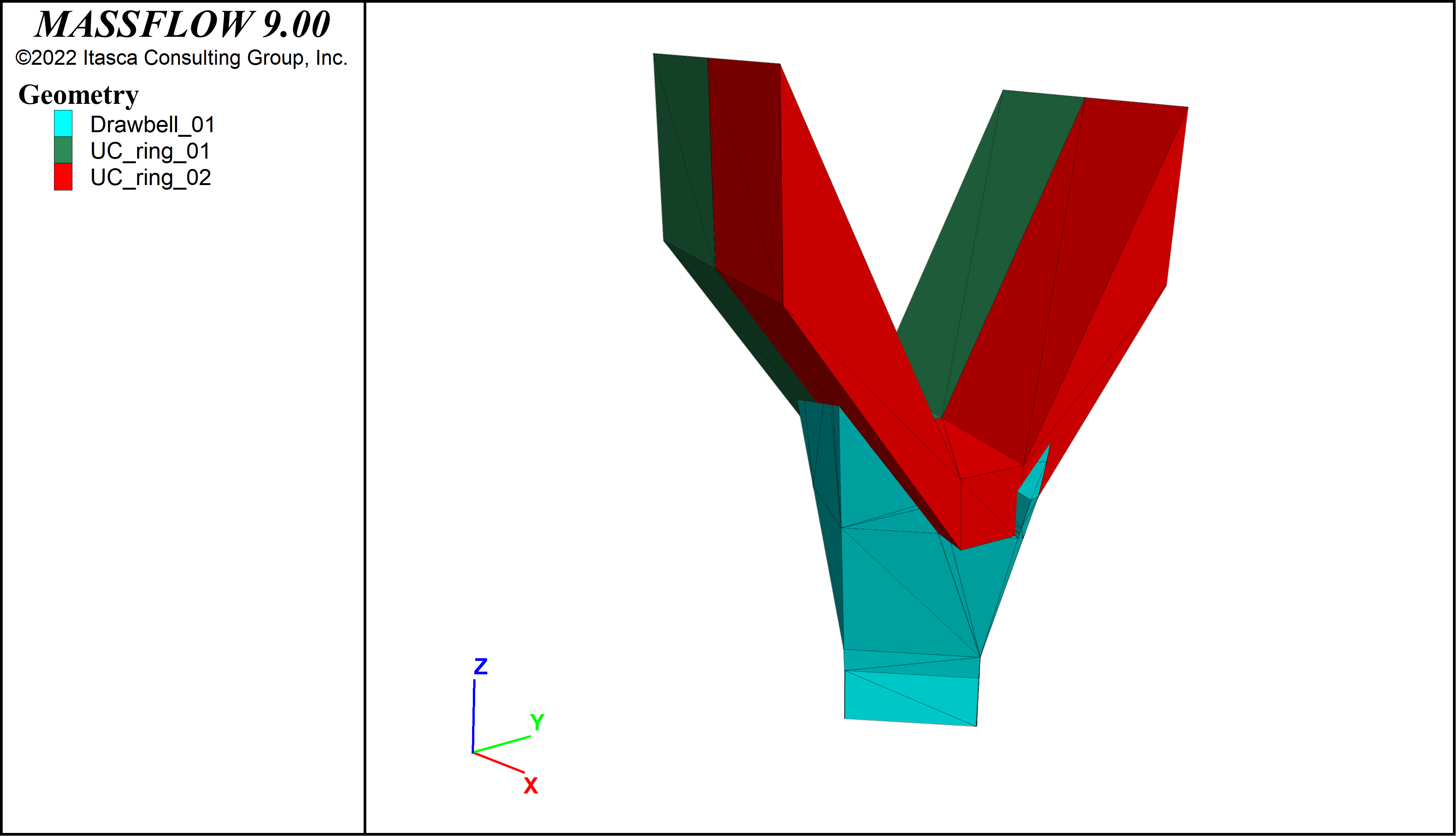
Figure 1: Geometry of gravity flow example with open pit.
For demonstration purposes, the proposed mining plan considers an extraction of 300 m of the material above the footprint. The objective is to study how gravity flow changes under different scenarios, such as:
Extraction sequencing of the material: Block vs. Panel caving
Ore fragmentation: Fine, Medium, and Coarse
Drawpoint spacing: 30x15, 32x20 and 34x24 drawpoint configurations
Mechanisms use: Fines migration application
Surface topography conditions: Flat and open pit
A total of 11 different examples are presented in the document, assembled in 5 comparative analyses. The rock mass properties and grade characteristics used in the examples are summarized in Table 1.
Property |
Unit |
Value |
|---|---|---|
Friction |
degrees |
40 |
Porosity |
% |
30 |
Mean Density |
\(t/m^3\) |
2.67 |
Ore Grade (Cu) |
% |
1.00 |
Dilution Grade |
% |
0.00 |
The different scenarios of fragmentation to the model are presented in Table 2. Fragmentation data is also included in the block model.
Parameter |
Unit |
Fine |
Medium |
Coarse |
Ultra-fine |
|---|---|---|---|---|---|
Material |
Ore |
Ore |
Ore |
Dilution |
|
\(P_{80}\) |
m |
0.3 |
1.1 |
1.7 |
0.02 |
Mean Diameter (\(P_{50}\)) |
m |
0.2 |
0.8 |
1.4 |
0.01 |
\(\alpha\) (Weibull shape parameter) |
0.89 |
2.66 |
3.32 |
3.32 |
|
\(\beta\) (Weibull scale parameter) |
m |
0.18 |
0.89 |
1.56 |
0.02 |
The designed dimensions for the drawbells are shown in Table 3. The dimensions are described in Draw Bells.
Dimension |
Unit |
Value |
|---|---|---|
Drawbell Type |
Conical |
|
Draw Drift Width |
m |
4.5 |
Draw Drift Height |
m |
4 |
Drawbell Height |
m |
16 |
Wall Angle |
deg |
71 |
The three drawpoint spacing configurations are presented in the figures below
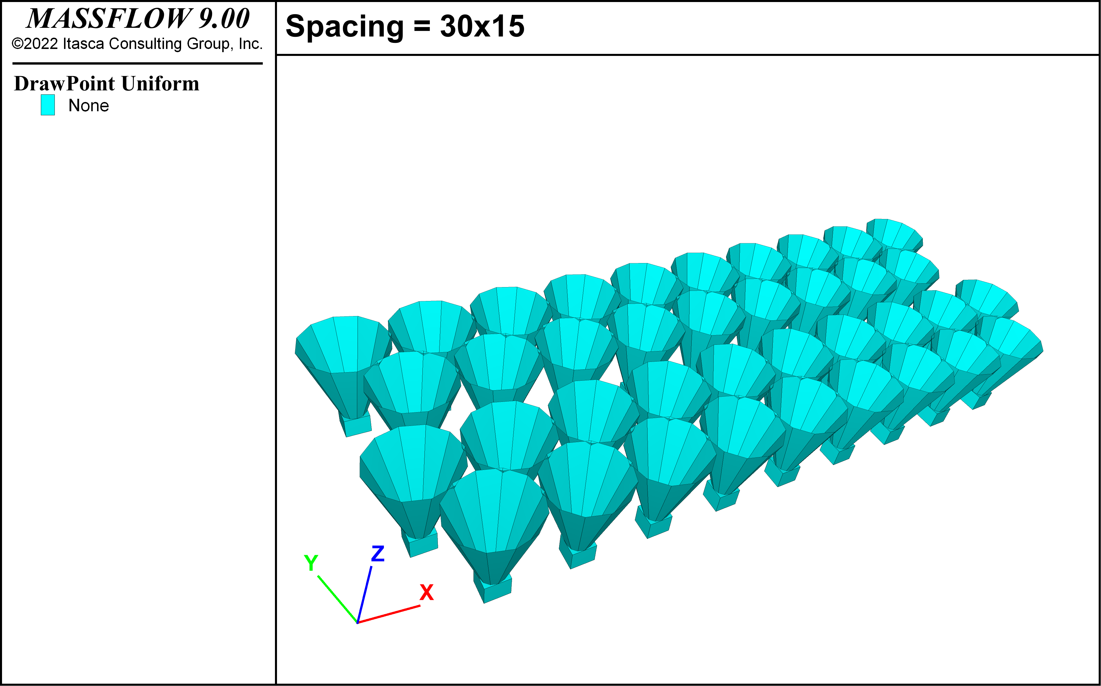
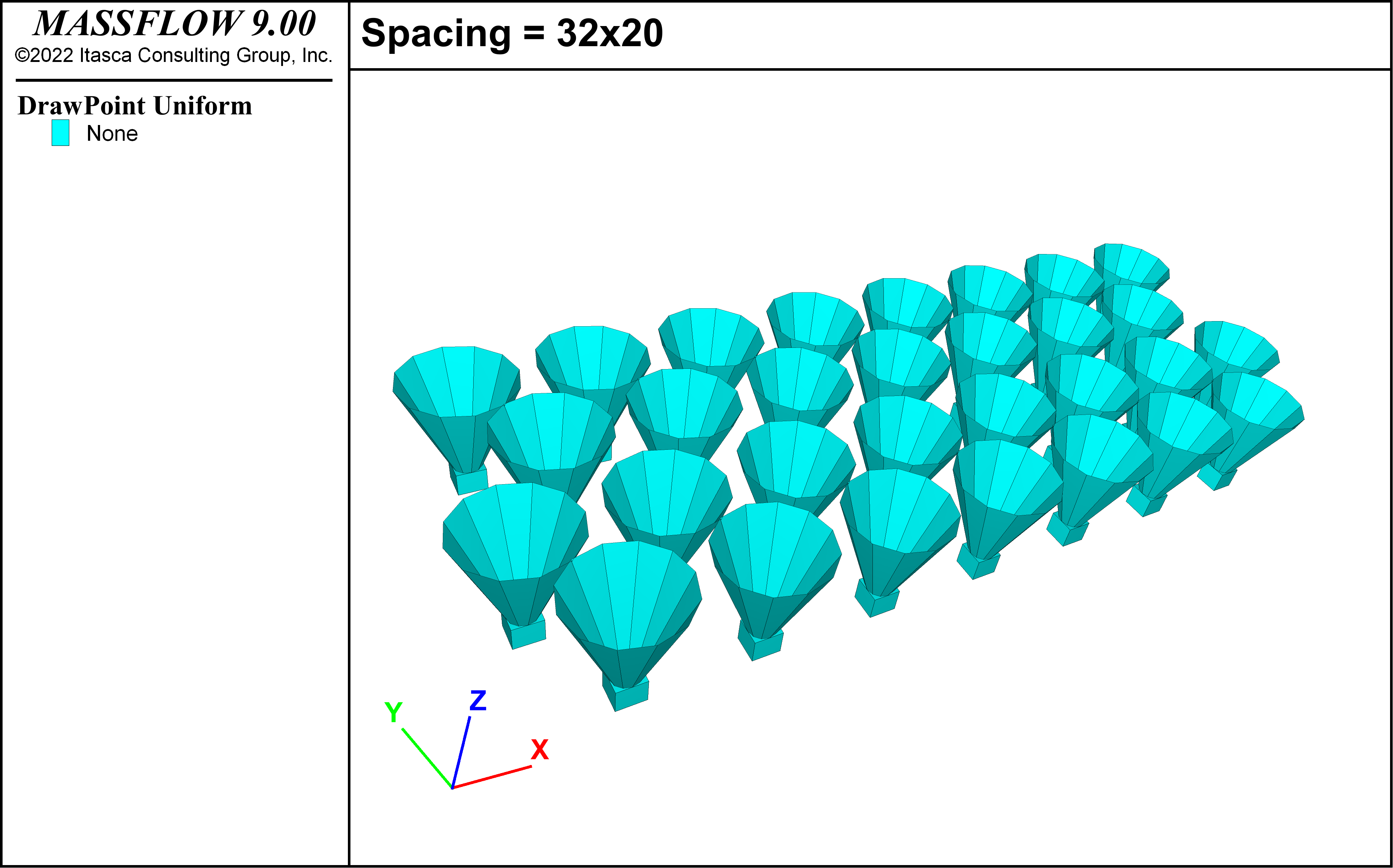
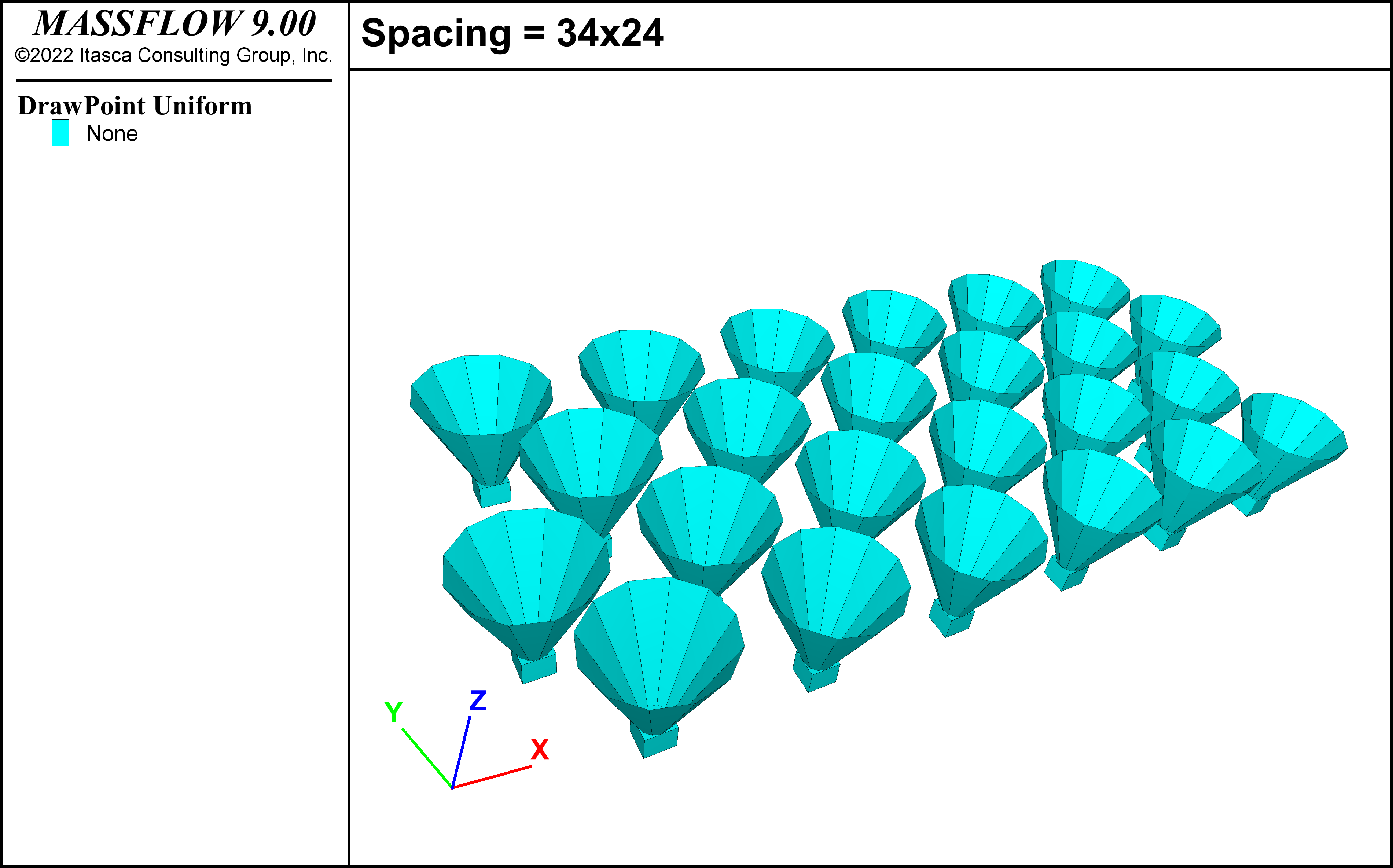
Figure 2: Drawpoint spacings.
Dilution content is used in some scenarios to assess the differences between cases. This variable is the percentage of waste material identified in the total material extraction as defined in (1)
Modeling Procedure
The scenarios presented in the problem statement lead to a total of eleven cases to be modeled in MassFlow. Each of the examples requires 4 data files, including:
Drawpoint locations: ”drawpoints.txt”
Drawpoint geometries: ”drawbells.txt”
Drawpoint extractions: ”drawperiod.txt”
Block model: ”mineBlocks.txt”
All the examples can be executed using the same data file “run.dat” as shown in Data Files.
Results and Discussion
As mentioned above, a total of eleven examples were modeled using MassFlow, five comparative analyses were made after running all examples. Table 4 shows a summary of the cases analyzed. Some of the examples are used multiple times to compare different aspects in MassFlow.
Example |
Comparative Analysis |
Extraction Sequence \(^1\) |
Drawpoint Spacing (m x m) |
Ore Fragmentation |
Fine Migration |
Surface |
|---|---|---|---|---|---|---|
1 |
1 |
BC |
30 x 15 |
Medium |
No |
Open pit |
2 |
1 & 2 |
PC |
30 x 15 |
Medium |
No |
Open pit |
3 |
2 & 3 & 4 |
PC |
30 x 15 |
Medium |
Yes |
Open Pit |
4 |
3 |
PC |
30 x 15 |
Fine |
Yes |
Open Pit |
5 |
3 |
PC |
30 x 15 |
Coarse |
Yes |
Open Pit |
6 |
4 |
PC |
32 x 20 |
Medium |
Yes |
Open Pit |
7 |
4 |
PC |
34 x 24 |
Medium |
Yes |
Open Pit |
8 |
5 |
PC |
32 x 20 |
Medium |
Yes |
Open pit (East) |
9 |
5 |
PC |
32 x 20 |
Medium |
Yes |
Open pit (West) |
10 \(^2\) |
5 |
PC |
32 x 20 |
Medium |
Yes |
Open pit |
11 \(^2\) |
5 |
PC |
32 x 20 |
Medium |
Yes |
Flat |
\(^1\) BC: Block Caving, PC: Panel Caving
\(^2\) Extended cases
The following sections describe each of the five comparative analysis
Comparison 1: Mine Sequencing
The following comparative analysis considers Examples 1 and 2, listed in Table 4. The objective, in this case, is to compare how the sequence of material extraction can change the way that mineral and dilution mixes and enter drawpoints.
While in Example 1 all drawpoints were open and the material was extracted at the same time from all drawpoints, representing a block caving mine, Case 2 started the extraction of material progressively from left to right, representing a panel caving mine. At the end of the execution of example plan 2, all the drawpoints were opened. Figure 3 shows that the total extraction was conducted for each case in a total of 12 periods of 120 days.
This plot was created by using the command massflow record to record the period mass for all drawpoints in the two examples. The table from Example 1 was then exported and imported into Example 2 for comparison.
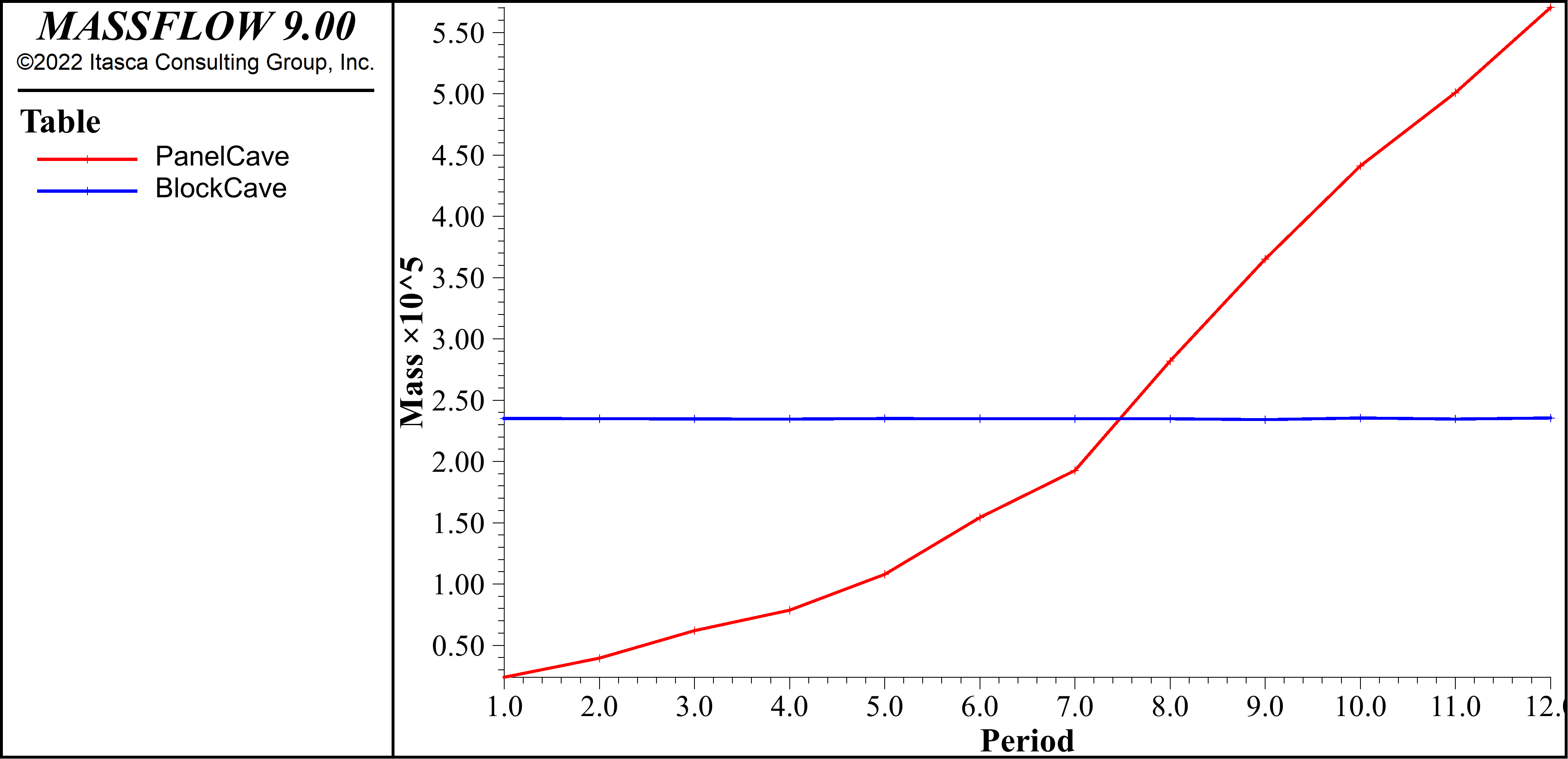
Figure 3: Total extraction for Example 1 (blue) and Example 2 (red) – Sequence comparison.
In both examples, approximately a total of 2.8 Mton were extracted from 38 drawpoints. Drawpoint spacing and material fragmentation curves are common, 30 x 15 and medium (\(P_{80}\) = 1.1 m) respectively.
The outcomes for both models are presented in Figure 5, where markers allow observing the movement of the remaining material after the extraction. Ore material is depicted with blue and dilution with red.
In Example 1, drawpoints did not report dilution before the first 12 periods. And, as it can be seen in Figure 4 dilution goes down evenly throughout the footprint. A different outcome is observed in Example 2, Figure 5, where dilution is reported in drawpoints that opened at the start of the plan.
These plots were created by plotting Mine Blocks, choosing Dilution as the label and adding a cut plane. Markers were then plotted, also with Dilution as the label and a clip box was added to only plot the markers close to the cut plane.
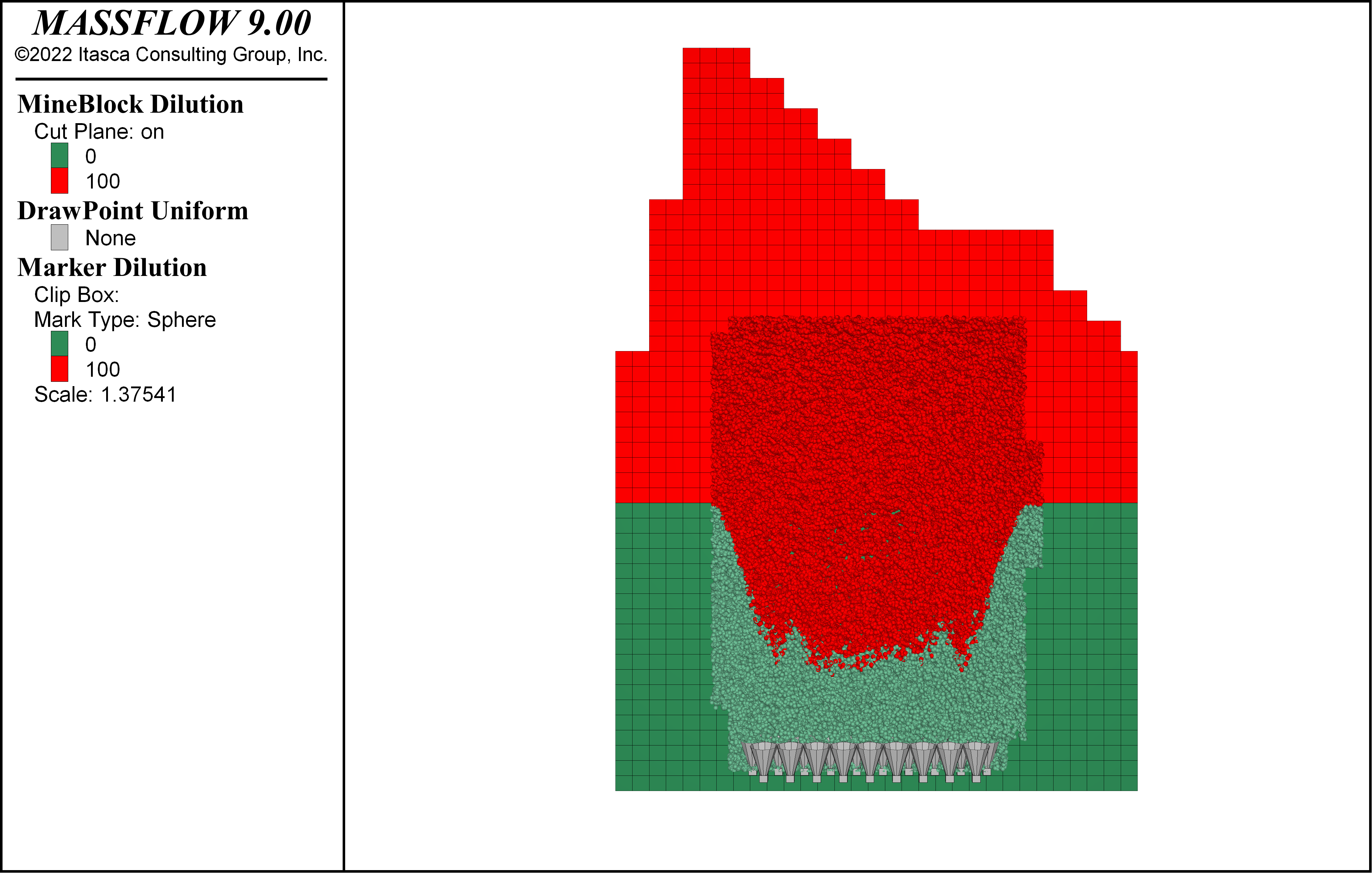
Figure 4: Dilution plot for Example 1 (block cave).

Figure 5: Dilution plot for Example 2 (panel cave).
Comparison 2: Ultrafine in dilution and fine migration mechanism
The next analysis compares the application of the fine migration mechanism in MassFlow, Examples 2 and 3 listed in Table 4. Dilution size fragmentation is considered medium (\(P_{80}\) = 1.1 m) in Example 2 and Ultra-fine (\(P_{80}\) = 0.02 m) in Example 3.
In both examples, approximately a total of 2.8 Mton are extracted from 38 drawpoints sequentially from left to right as a panel caving mine in 12 periods of 120 days. Drawpoint spacing and ore fragmentation are common to both cases, 30 m x 15 m and medium (\(P_{80}\) = 1.1 m), respectively.
The outcomes for the models are presented in Figure 6 and Figure 7, where markers show the movement of the remaining material after the extraction. In this case, colors represent the original position of the material.
In Example 2 (Figure 6), material descends regularly according to the extraction performed. In Example 3, the combination ultrafine dilution + fine migration is activated, meaning that material can percolate from higher positions and reaches drawpoints in less time. This is clear in Figure 7, where red material (higher located material) percolates through the column and reaches drawpoints. Furthermore, it is possible to observe how fine migration activation generates a different mix of the material through the column.
These plots were created by contouring the mine blocks and markers by Height and modifying the contour limits and interval to achieve a small number of color. A geometry of a plane was created and plotted to show the original dilution height.
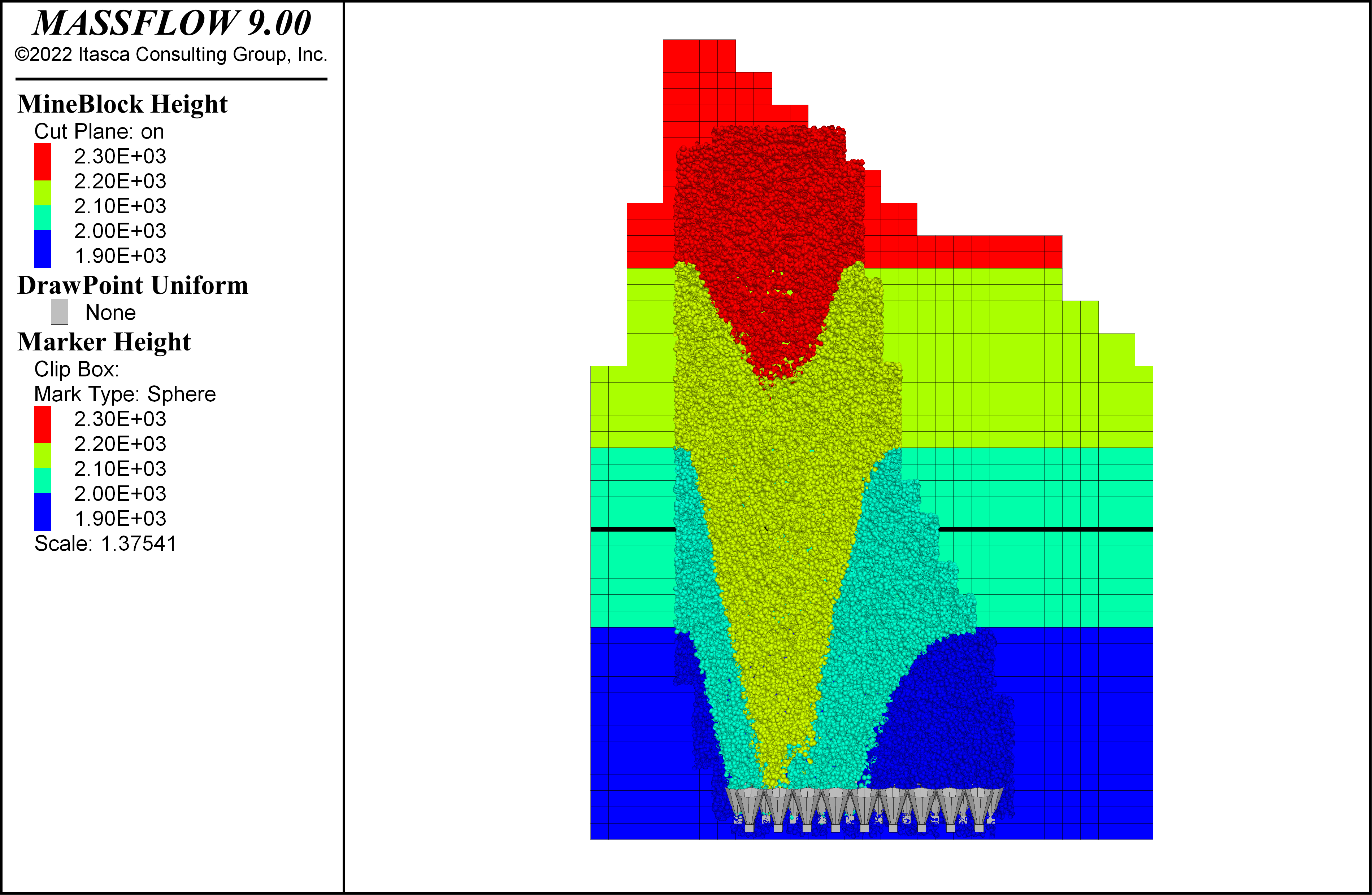
Figure 6: Origin of material for Example 2. The original dilution height is shown by a thick black line.
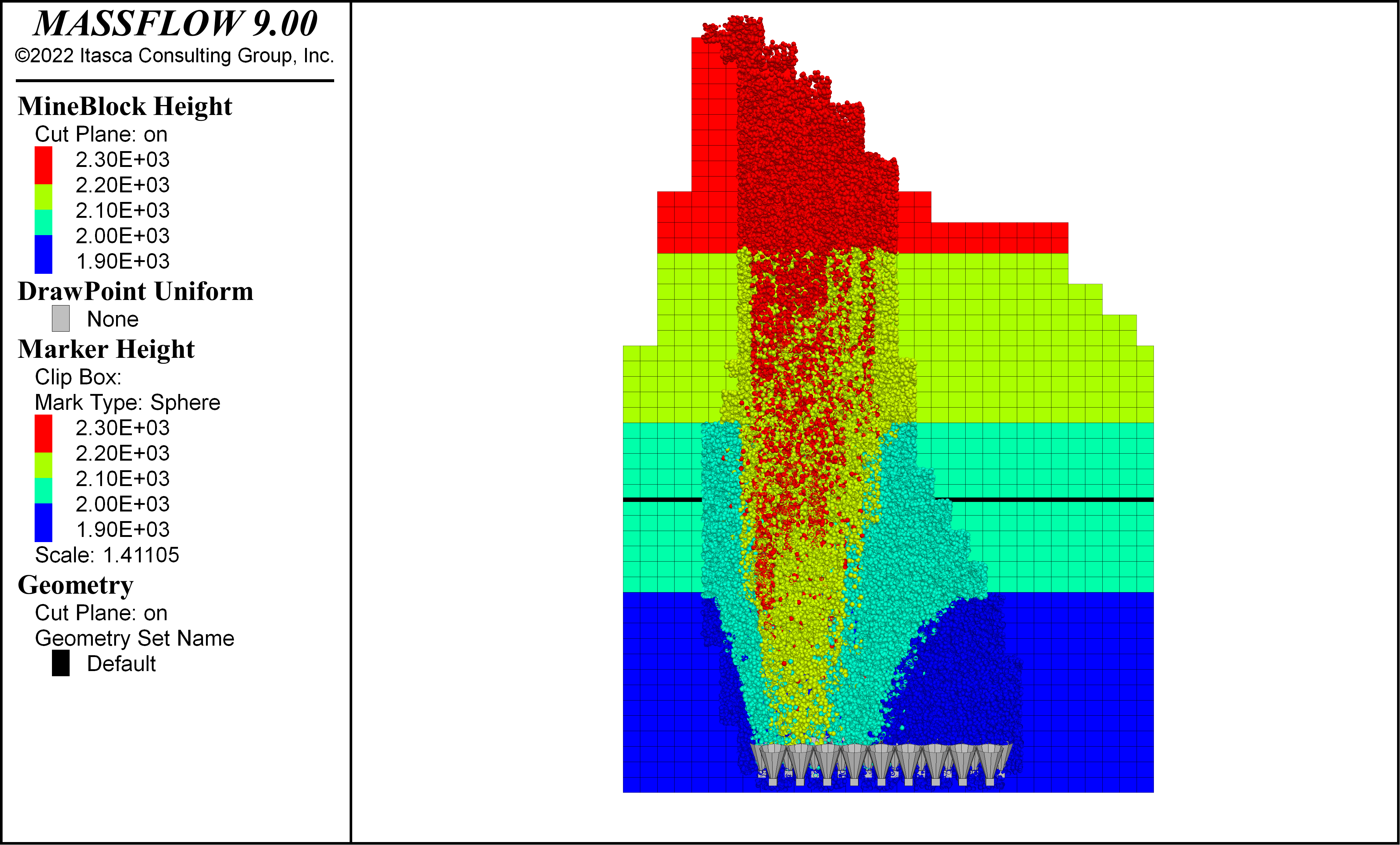
Figure 7: Origin of material for Example 3 (ultra-fine dilution + fine migration). The original dilution height is shown by a thick black line.
Comparison 3: Effect of Fragmentation
The third comparison explores the influence of ore fragmentation in gravity flow modeled in MassFlow for three sizes; medium (\(P_{80}\) = 1.1 m), fine (\(P_{80}\) = 0.3 m), and coarse (\(P_{80}\) = 1.7 m), that is, Examples 3, 4, and 5 respectively, listed in Table 4.
Extraction sequence and drawpoint spacing are common to these cases: panel caving type and 30 m x 15 m, respectively. Dilution is considered as ultra-fine fragmentation (\(P_{80}\) = 0.02 m). The fines migration mechanism is activated.
A comparison between the outcomes is presented in Figure 8, Figure 9, and Figure 10, where markers show the movement of the remaining material after the extraction. From top to bottom: fine, medium, and coarse fragmentation results are shown.
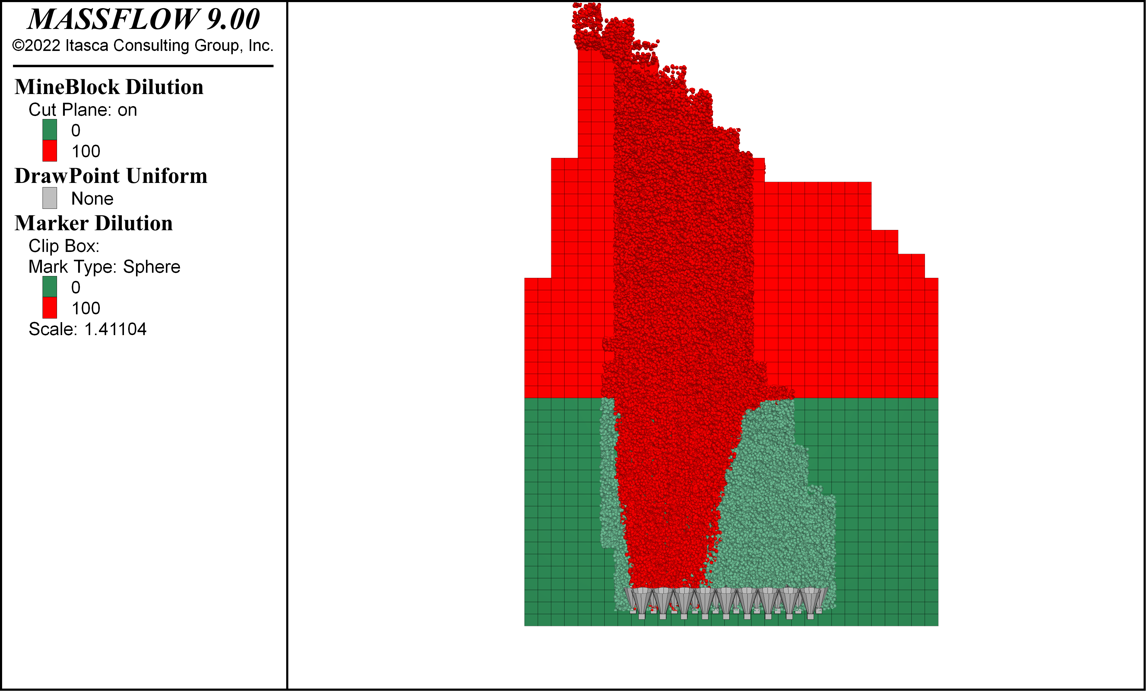
Figure 8: Dilution plot for Example 4 (fine fragmentation).
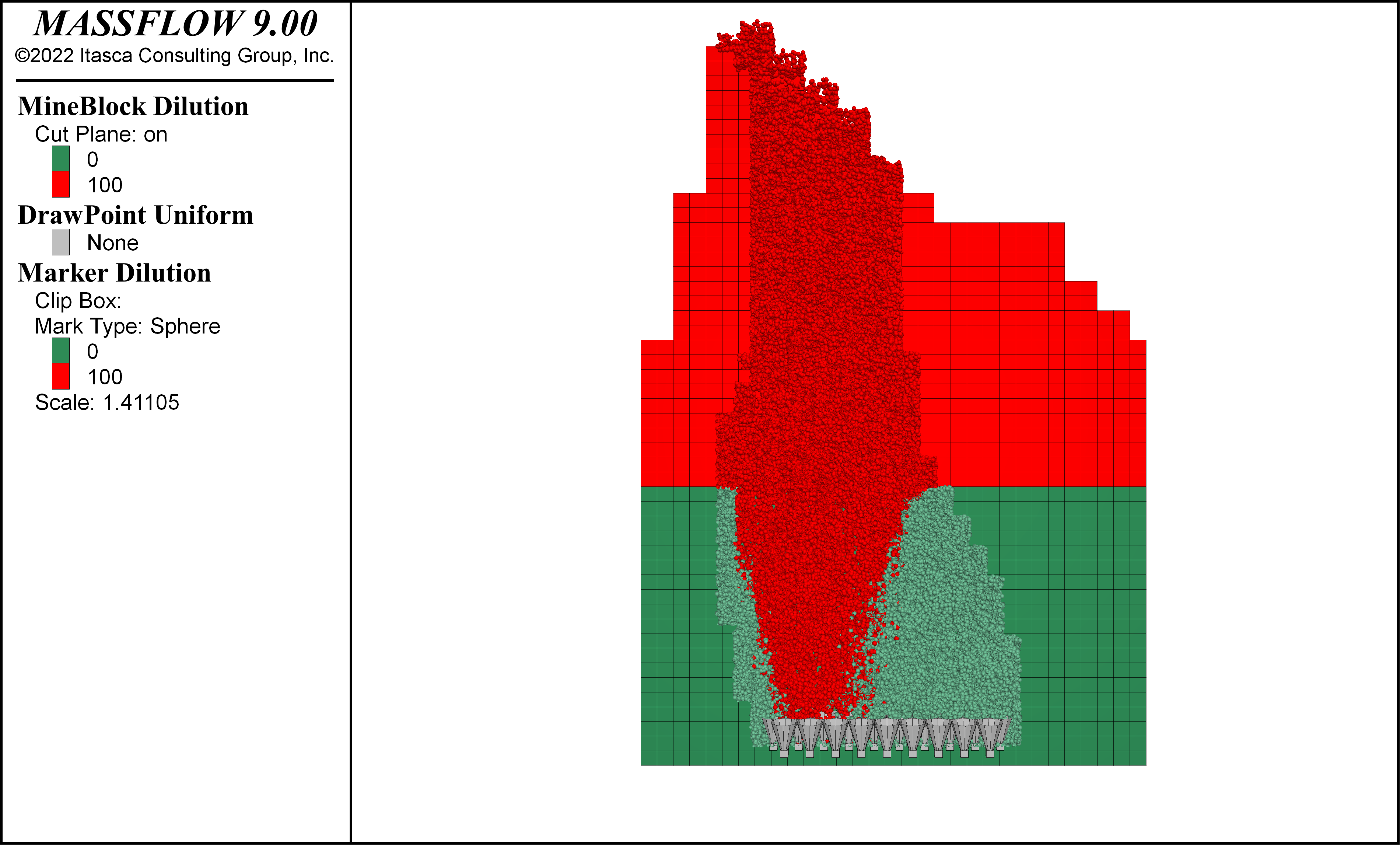
Figure 9: Dilution plot for Example 3 (medium fragmentation).
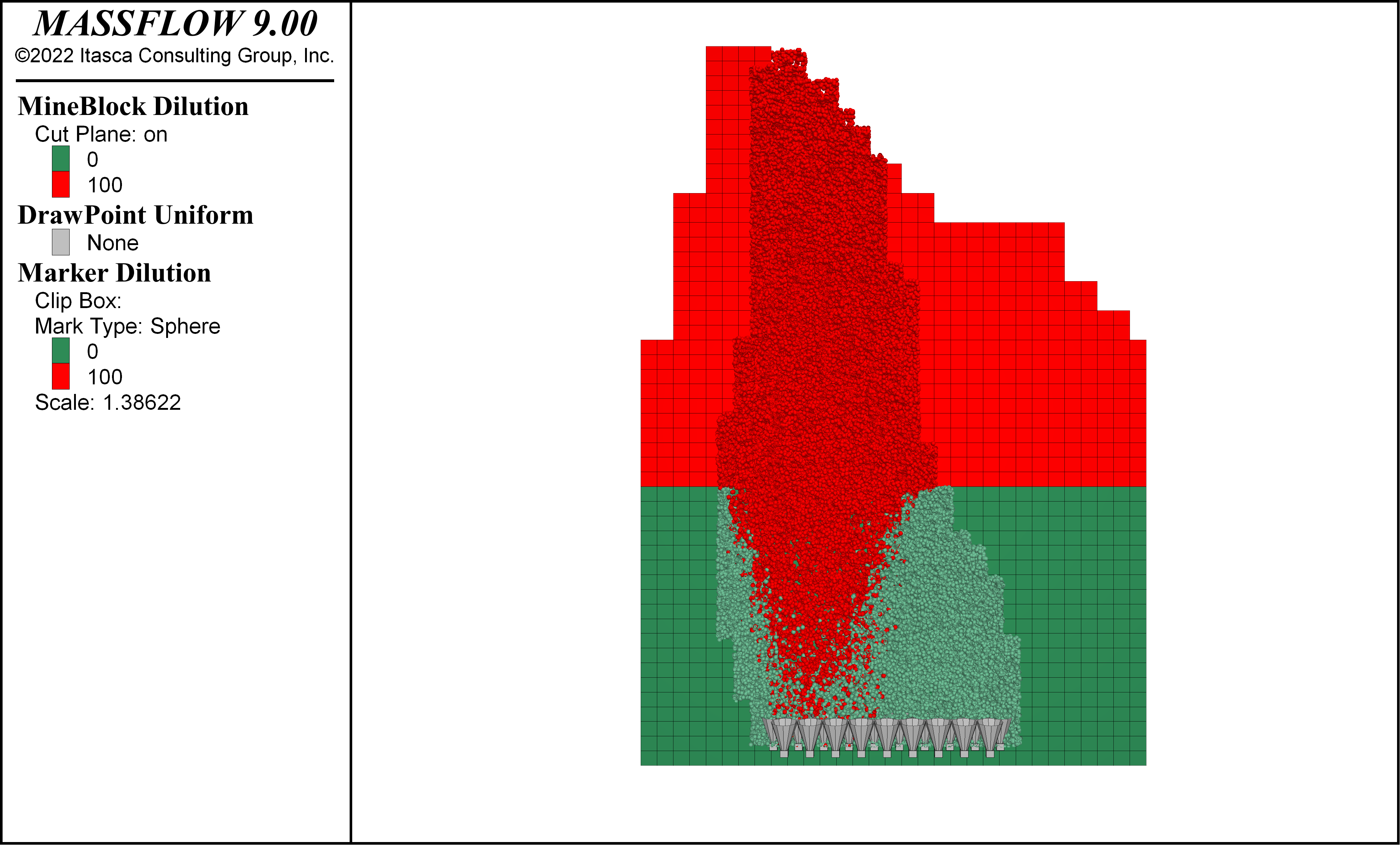
Figure 10: Dilution plot for Example 5 (coarse fragmentation).
Figure 11, Figure 12, and Figure 13 present views of the Isolated Movement Zones (IMZs) for each scenario. From top to bottom, it is observed how the amount of mobilized fines increases when the ore is coarser.
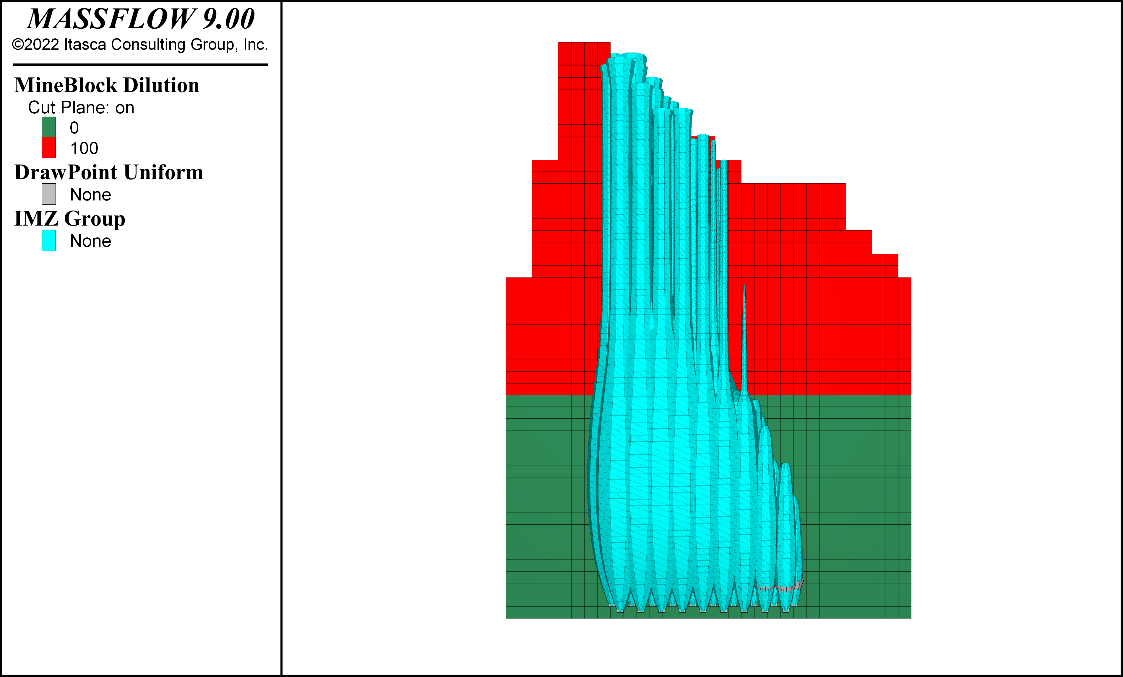
Figure 11: Isolated Movement Zone plot for Example 4 (fine fragmentation).

Figure 12: Isolated Movement Zone plot for Example 3 (medium fragmentation).
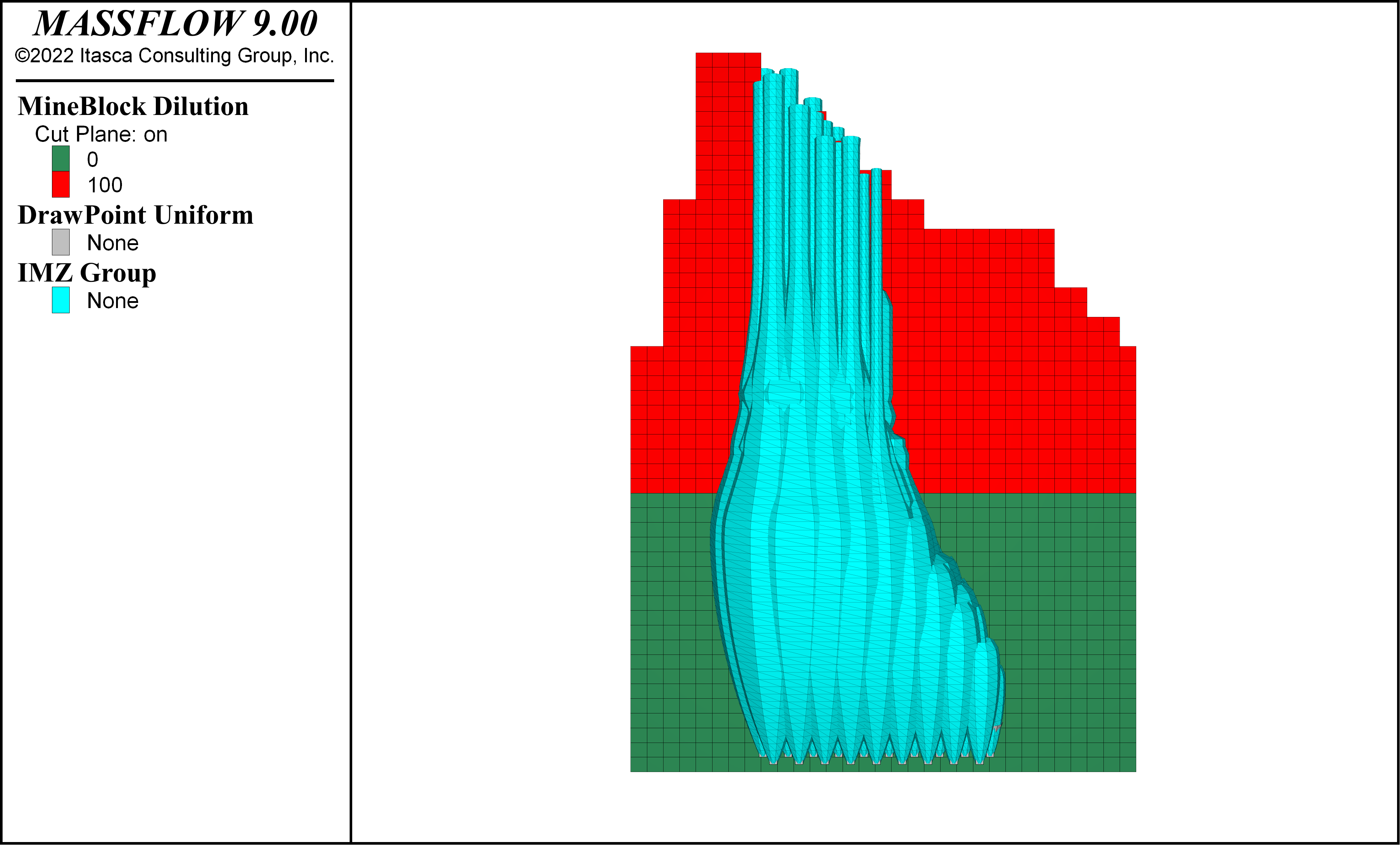
Figure 13: Isolated Movement Zone plot for Example 5 (coarse fragmentation).
Comparison 4: Drawpoint Spacing
This comparative analysis considers Examples 3, 6, and 7 as listed in Table 4, from smallest to largest drawpoint spacing, respectively. The objective, in this case, is to compare how the distance between drawpoints can alter the way that mineral and dilution mixes and enters drawpoints.
To keep the area of the footprint and the total mineral extraction, the number of drawpoints changes along with the drawpoint spacing ( Table 5). The distribution of drawpoints for each case is shown in Figure 2.
30 x 15 (m x m) |
32 x 20 (m x m) |
34 x 24 (m x m) |
|
|---|---|---|---|
Number of Drawpoints |
34 |
32 |
24 |
Extraction sequences are common to all three models with slightly different tonnage in drawpoints to keep the proportion. Assigned ore fragmentation is medium (\(P_{80}\) = 1.1 m), and dilution fragmentation is ultrafine (\(P_{80}\) = 0.02 m). The fine migration mechanism is activated.
Figure 14 shows the outcomes, where dilution content (defined previously in (1)) is compared for the three drawpoint spacings. It is observed that dilution enters earlier in the larger drawpoint spacing. In medium and smaller drawpoint spacing dilution entry is similar through the periods.
This behavior is due to the combination between drawpoint spacing and fragmentation. Because in Example 7 drawpoints are widely spread out, the IMZs do not interact with each other. Without IMZ interaction, gravity flow is mainly vertical and dilution is reached faster than in the previous two cases.
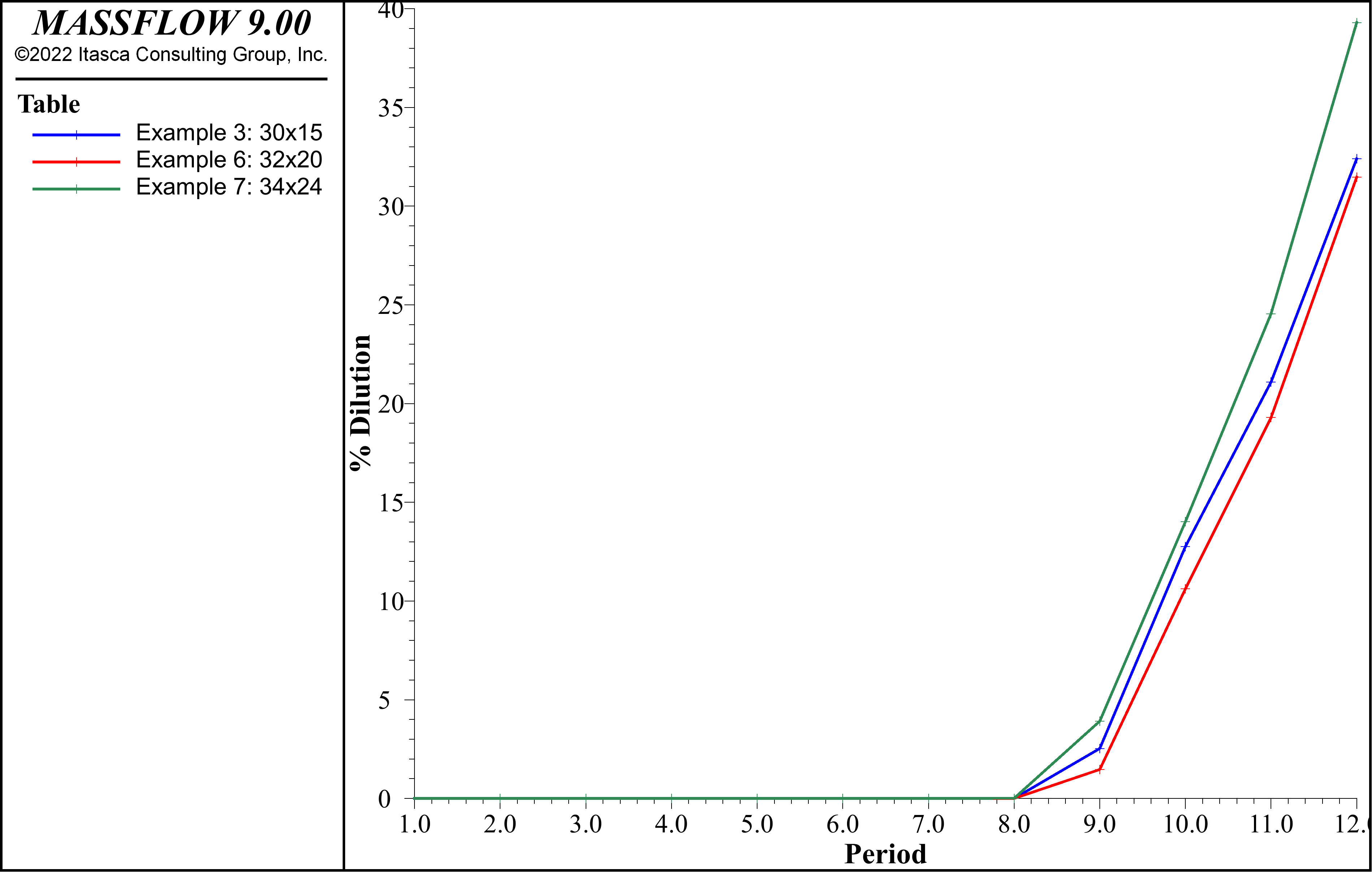
Figure 14: Dilution content per period for different drawpoint spacings.
Figure 15, Figure 16, and Figure 17 present the visual results of MassFlow in the last period of extraction. While in Examples 3 and 6 dilution material is scattered through the columns, in example 7 dilution has entered in the first half of the footprint.
Figure 15: Dilution plot for Example 3 (30 x 15).

Figure 16: Dilution plot for Example 6 (32 x 20).
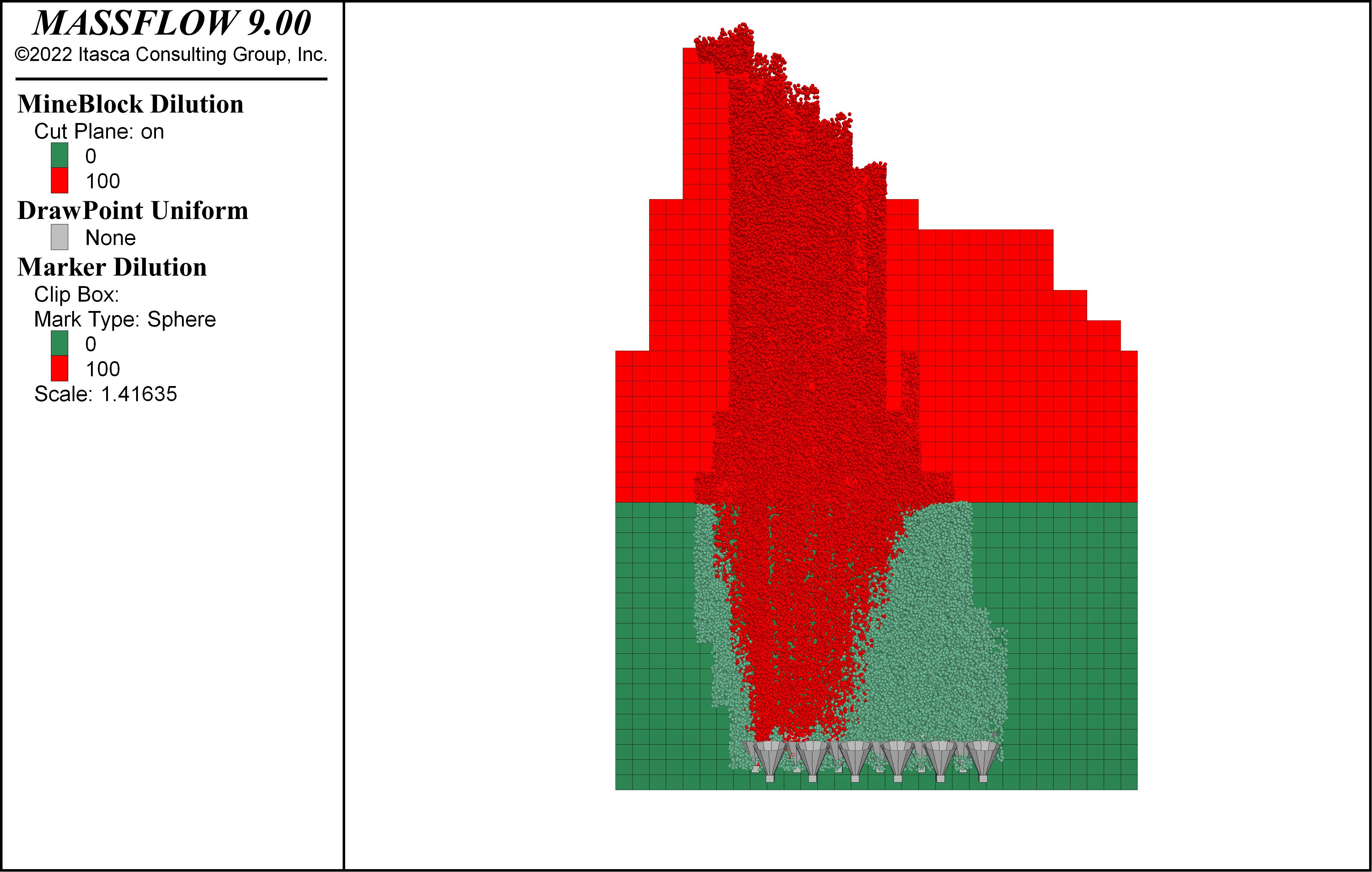
Figure 17: Dilution plot for Example 7 (34 x 24).
Comparison 5: Topography Conditions
The last comparison developed explores the influence of the topography above the underground mine. The scenarios consider an open pit mine presence in one case and a flat surface ground in the other.
Extraction sequences are common in the two cases, where the drawpoint spacing is 32 m x 20 m. Assigned ore fragmentation is medium (\(P_{80}\) = 1.1 m), and dilution fragmentation is ultrafine (\(P_{80}\) = 0.02 m). The fine migration mechanism is activated.
Both cases present the same sequencing and extraction profile, with only the surface varying, which in this case corresponds to the East and West walls of a pit.
Figure 18 and Figure 19 show the impact on dilution by having a sequencing that advances from the center of the pit (West wall) or towards the center of the pit (East wall), resulting in the latter option being more disadvantageous, given that a greater amount of dilution is reported. This is emphasized further in Figure 20.
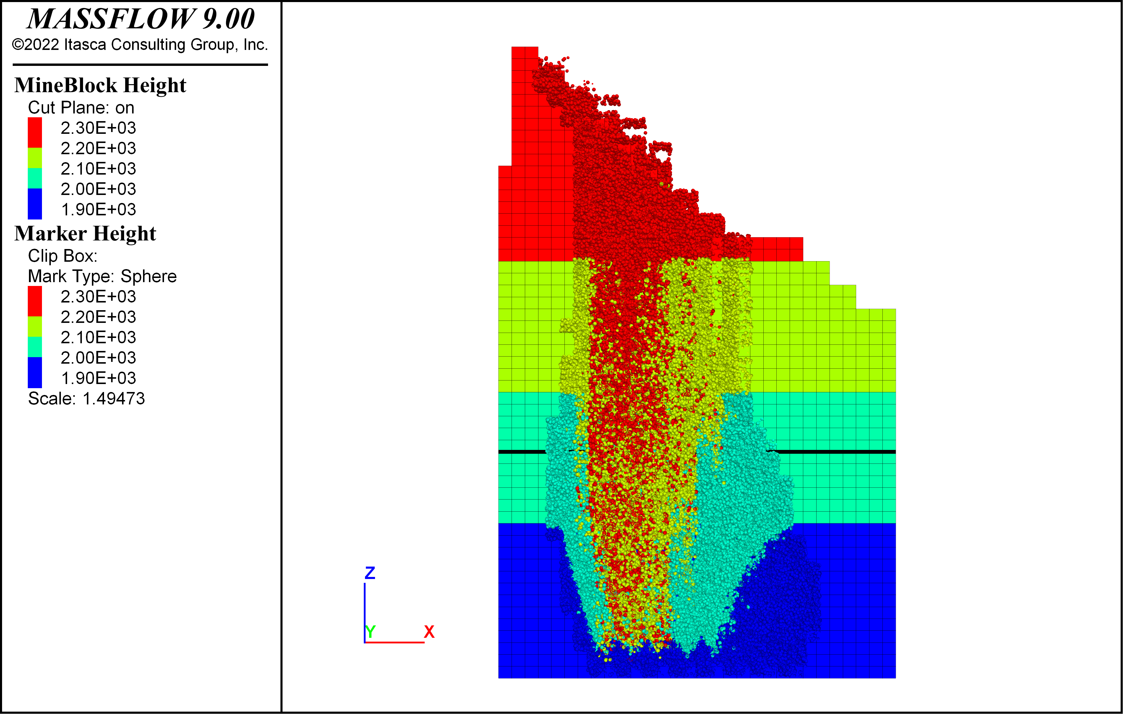
Figure 18: Origin of material for Example 8 (East).

Figure 19: Origin of material for Example 9 (West).
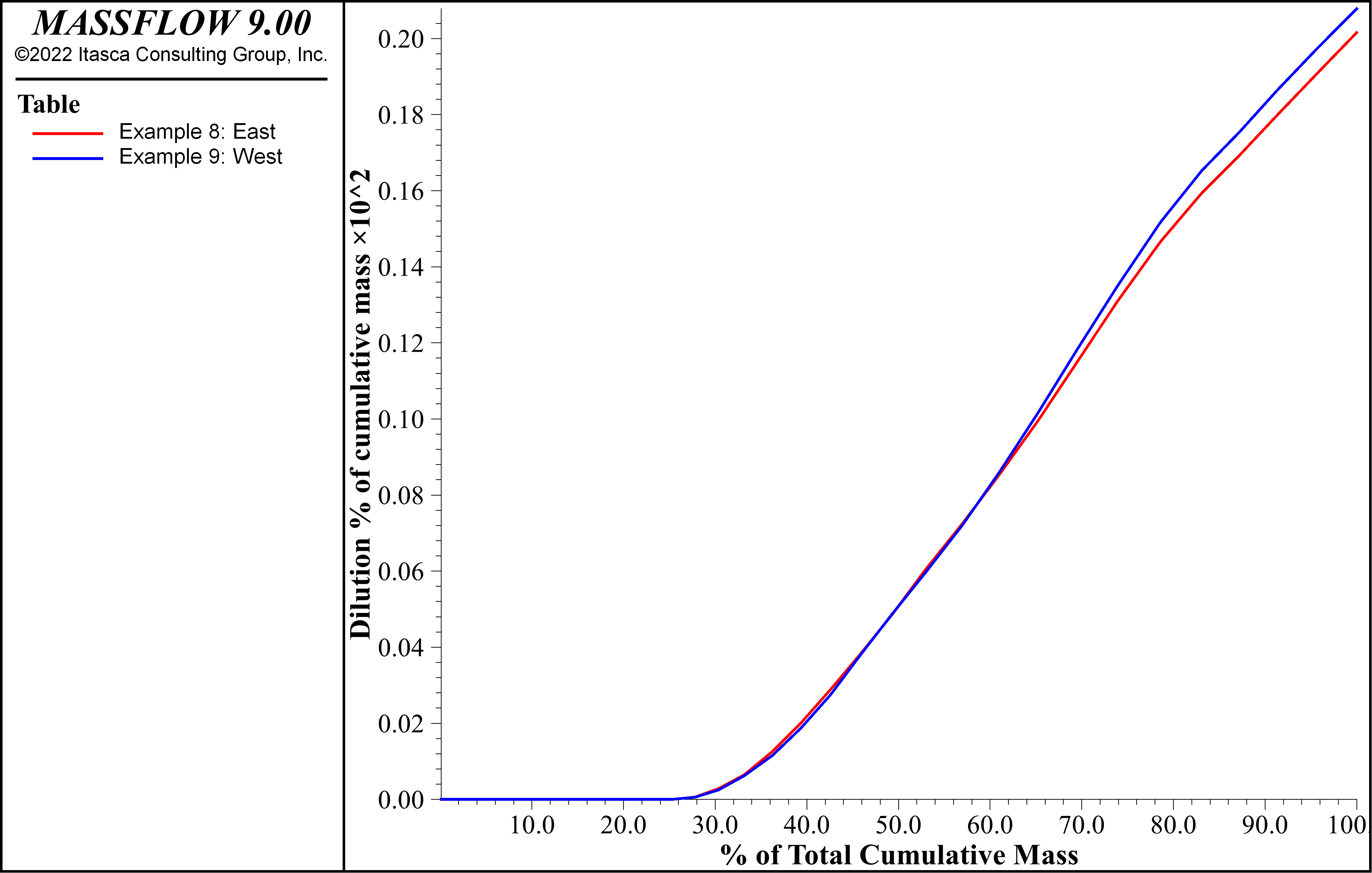
Figure 20: Cumulative dilution [%] versus cumulative tonnage [%] for examples 8 and 9.
Effect of dilution with and without pre-existing pit
The following examples visualize the impact of the presence of a pre-existing it. The extraction horizon is larger than in the previously reviewed examples. The boundary conditions are detailed below.
Extraction time: 15 years
Extraction points: 88
Extraction mesh: 32 x 20 [m x m]
Mineralized rock fragmentation: \(P_{80}\) = 1.1 [m]
Dilutent fragmentation: \(P_{80}\) = 0.02 [m]
Extraction column 300 [m] (on it dilutent material)
Both cases correspond to extraction advancing in an EW direction, but, as can be seen in Figure 21, the dilution extraction mechanism is vertical.
On the other hand, Figure 22 shows the impact that the pit has on the entry of the dilution, given that, in this case, the dilution entry mechanism is lateral, coming from the displacement of the broken material towards the bottom of the pit, a product of its walls.
In addition, in Figure 23 it can be concluded that in the presence of the pit, once the extraction advance reaches the center of the pit, the amount of dilution reported jumps, unlike the case without the presence of the pit, which has a slightly more continuous behavior (Figure 23).
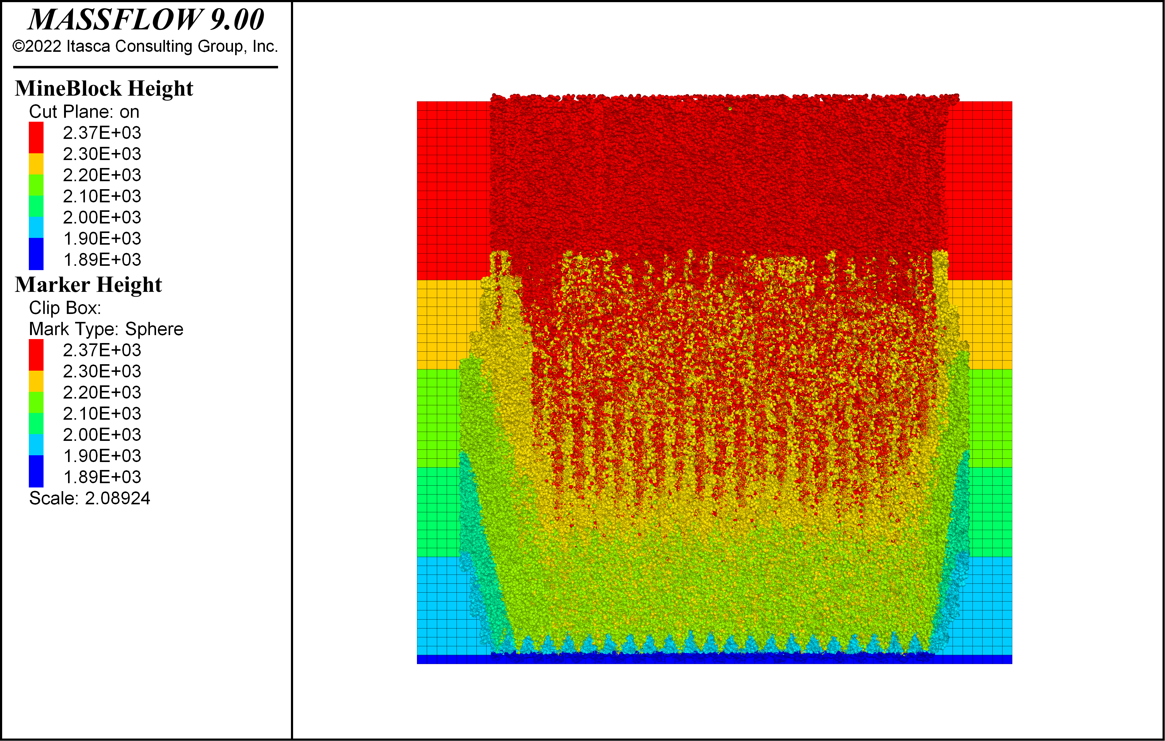
Figure 21: Origin of material for Example 11 (flat topography).
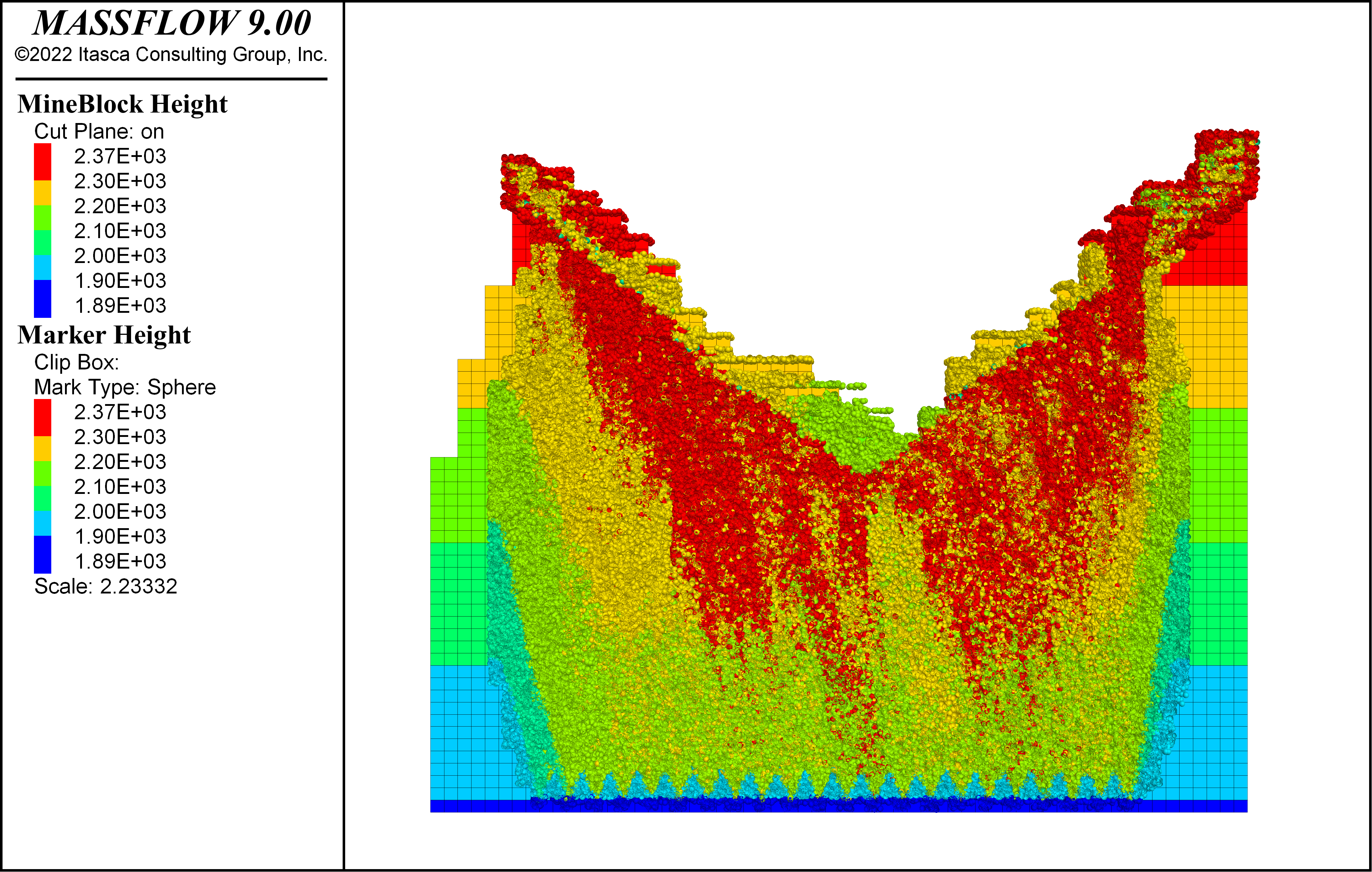
Figure 22: Origin of material for Example 10 (pit topography).
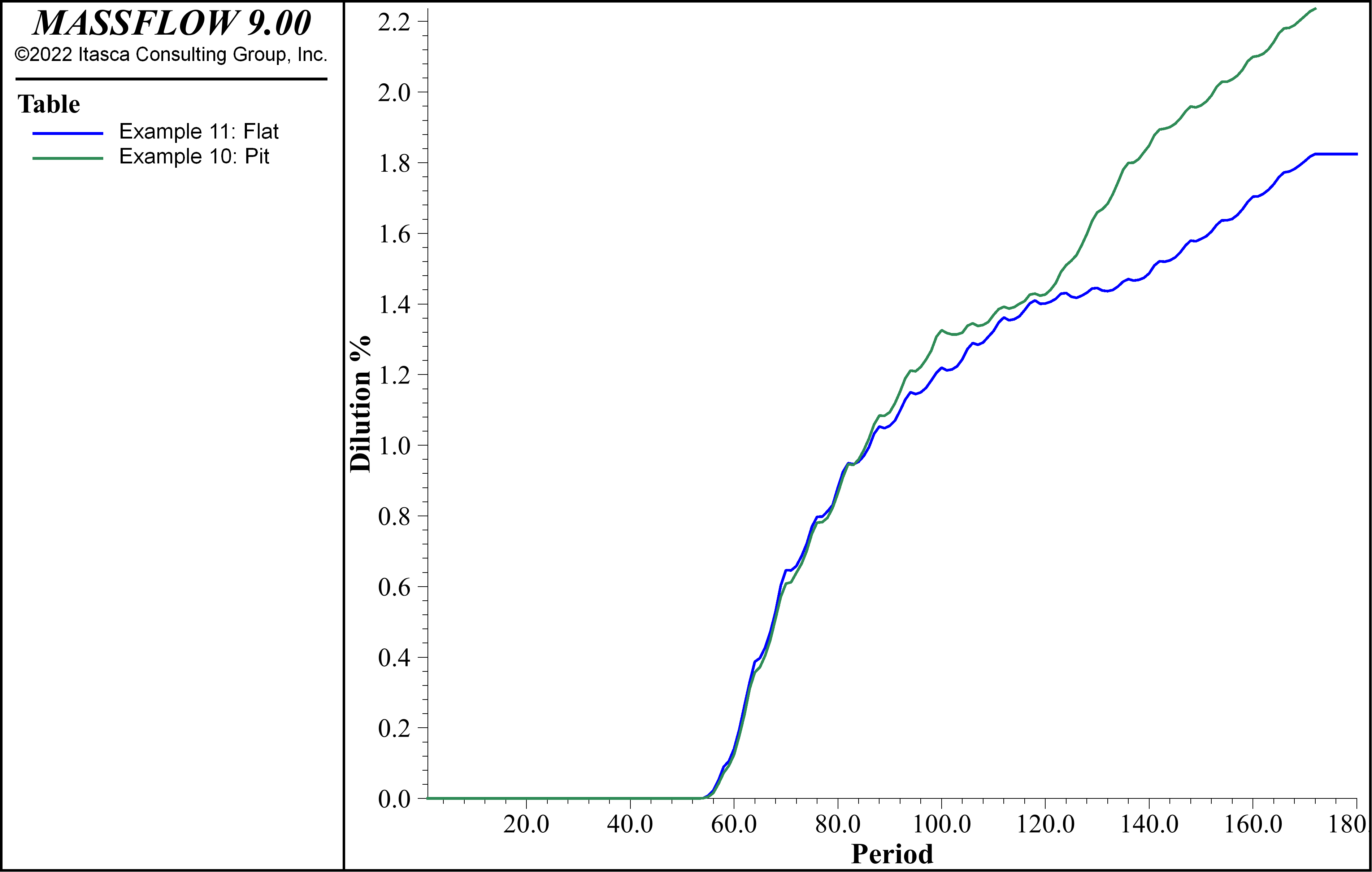
Figure 23: Cumulative dilution [%] versus cumulative tonnage [%] for examples 10 and 11.
Data Files
The data file for the base case is shown below. Other examples are variations of this.
Example1/run.dat
model new
model random 10000
;massflow mine-block import-txt "mineBlocks.txt"
;massflow drawpoint import-txt "drawpoints.txt"
;massflow drawpoint import-drawbell-txt "drawbells.txt"
;massflow drawpoint import-drawperiod-txt "drawperiod.txt"
massflow mine-block import "mineBlocks.csv"
massflow drawpoint import "drawpoints.csv"
massflow drawpoint import-drawbell "drawbells.csv"
massflow drawpoint import-drawperiod "drawperiod.csv"
massflow initialize layer-thickness 0.5 percent-empty 0.75 save-days 200 compute-days 1440
massflow marker initialize spacing 0.25
massflow marker report-days 720

massflow record name 'BlockCave'

massflow clean
massflow compute
massflow drawpoint extraction-report

; group mine blocks for plotting
massflow mine-block group 'Waste/Dilution' slot 'Type'
massflow mine-block group 'Ore' slot 'Type' range position-z 1880 2060

model save 'example1_final'

; export table
table 'BlockCave' export 'MassBlockCave.tab'
| Was this helpful? ... | Itasca Software © 2024, Itasca | Updated: Nov 12, 2025 |
