MassFlow Theory and Background
MassFlow is a gravity flow simulator that can be run on its own or coupled with FLAC3D or 3DEC to account for the influence of stress.
Background
REBOP
REBOP is a computer program that was developed by Itasca to emulate the flow behavior observed in PFC simulations of draw from block and panel caves, but much more rapidly and at the scale of entire panel or block (hence the name Rapid Emulator Based On PFC). To better understand the mechanics of flow, a series of large-scale physical draw experiments were conducted at the Julius Kruttschnitt Mineral Research Centre (JKMRC) at the University of Queensland, Australia. The purpose was to measure the height and width of the Isolated Movement Zone (IMZ), the volume of material that moves above a drawpoint in response to draw (Figure 1).
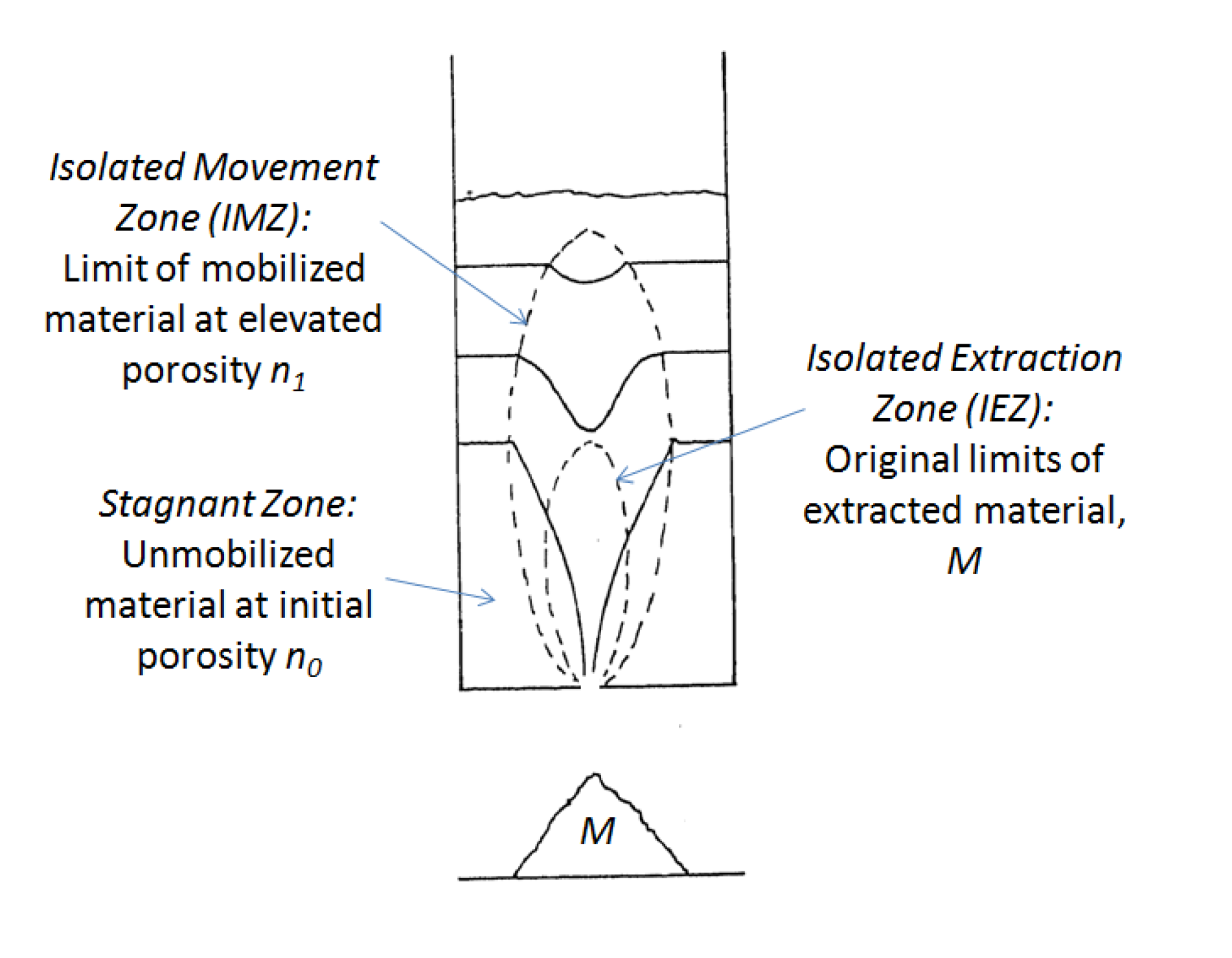
Figure 1: Volumes associated with extraction of material from an isolated drawpoint (adapted from Alford 1978).
A detailed review of IMZ shape data from other existing physical modeling data and from kinematic theory was conducted by Itasca in parallel. When assembled together with the original PFC IMZ shapes in a single graph and expressed in terms of fragment size, all of the IMZ data exhibited a correspondence that had not previously been recognized. The graph ( Figure 3) indicates that much of the physical and numerical modelling data are consistent with Nedderman’s 1995 kinematic theory, which suggested that the IMZ width, \(W\), and height, \(H\), when expressed in mean fragment diameters, are related by \(W = 3.42\sqrt{H}\).
In parallel with this development, additional PFC simulations conducted by Itasca (combined with a review of available physical modelling data), revealed that the well-known drawdown profile internal to an IMZ (fast at the center, slow at the edges, as shown in Figure 1) was in fact controlled by the fragment size in a well-defined manner. The mechanisms controlling fines migration, and secondary fragmentation were also isolated and the importance of rilling on both the free surface and along internal cave boundaries was recognized. The REBOP logic was subsequently refined to reflect these new understandings and has since been optimized and further validated for cave-scale simulations of flow at several mines. For more detail on the basis for REBOP, see Pierce (2010).
MassFlow
MassFlow is a new code that improves on the concepts of REBOP. The flow theory behind MassFlow differs in some respects from previous understanding. Laubscher (1994) suggested that IMZs grow to a narrower finite diameter that is dependent upon the draw width and the fragment size distribution (Figure 2). Figure 3 compares these to the IMZ widths that are represented in MassFlow.
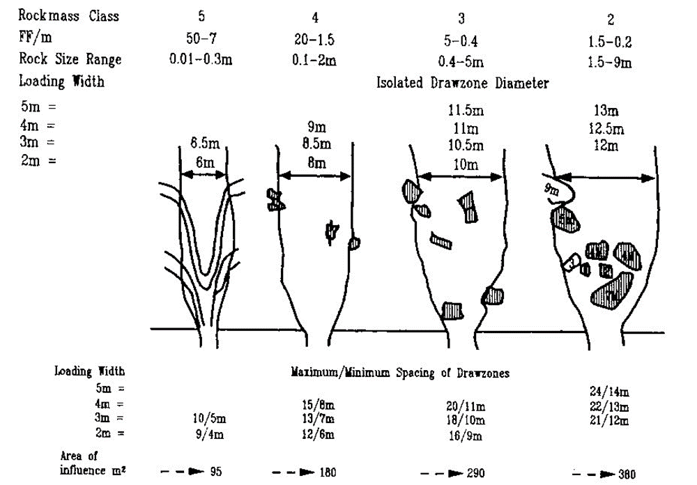
Figure 2: IMZ dimensions proposed by Laubscher (1994) based on in-situ observations of hang-ups and physical modelling data.
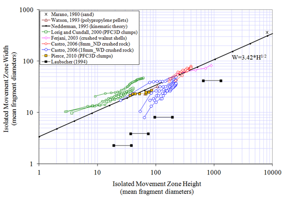
Figure 3: Comparison of IMZ width versus height from 3D experiments and simulations, the kinematic theory of Nedderman (1995) (solid line and equation) and the empirical model of Laubscher (1994).
The IMZ widths suggested by Laubscher for coarser materials are clearly much narrower and would in fact result in isolated draw for most modern caving layouts. Laubscher proposed that interactive draw, a mechanism in which the stagnant material between IMZs can be driven to stress-induced flow under specific draw conditions, was capable of mobilizing the material between IMZs, thus encouraging uniform drawdown even when IMZs do not touch. This mechanism can be clearly demonstrated in certain physical and numerical models of flow.
The large-scale physical modelling studies conducted at the JKMRC demonstrate, however, that the mechanism is not present when stresses are permitted to arch outside of the draw region (which is believed to often be the case in situ and is a matter of appropriate model boundary conditions). So, both interactive draw theory and overlapping draw theory (MassFlow) can result in the same outcome (uniform drawdown) but for very different reasons:
Interactive draw theory: Suggests narrow IMZs that would not overlap above modern drawpoint layouts (e.g. 30mx15m) but interactive draw mechanisms act to mobilize the intervening stagnant material to cause uniform drawdown.
Overlapping draw theory (MassFlow): Suggests wider IMZs that overlap above modern drawpoint layouts (e.g. 30mx15m). Interactive draw mechanisms not present in most cases and not required to achieve uniform drawdown.
Flow in MassFlow is kinematically controlled, i.e. material cannot be mobilized via stress-driven yielding and flow. Stress-driven flow may occur in caving scenarios where arching is inhibited (e.g. where a large weak fault parallels the cave boundary) or where an overlying pit slope or hangingwall fails, redistributing material due to collapse or by “pushing” material into the advancing cave. The potential for blockage of drawpoints (e.g. due to hangups) is currently not considered within MassFlow but is under development.
Formulation
The following formulation is extracted from Pierce (2010)
Mine Blocks
The initial state of the material in a MassFlow model is described by a user-generated three-dimensional array of blocks. The block array is fixed in space and aligned with a rectangular coordinate system (x,y,z), in which z is vertical and positive upward. Block size is constant, but can have different dimensions in each coordinate direction. Each block is defined by the user as a point in space corresponding to the center of the block and a unique ID. Blocks must be present throughout the volume in which flow is of interest. The top of the block array is assumed to be a free surface, and the sides and base of the array are assumed to be hard boundaries to flow.
IMZ Limits
An IMZ is represented by a series of horizontal disk-shaped layers. Material inside the disks has moved and is characterized by a dilated final porosity, \(n_1\), while the material outside the disk is stagnant and has a porosity, \(n_0\), that is less than or equal to the porosity inside the disk.
A single set of properties representative of the stagnant material are obtained by averaging the properties (derived from the block model) of 24 equally spaced points along the disk perimeter. The properties of the mobilized material inside the disk are obtained by averaging the properties of all markers contained within the disk. Markers are used to track material movements inside the IMZ.
The lowermost disk has an initial and fixed radius that is equal to half of the drawpoint width, and a base elevation equal to the draw drift back. Experimental evidence suggests that the center of the IMZ lies approximately one-half draw width into the drawbell.
The goal is to establish the change in IMZ size and shape resulting from extracting a given mass, \(\Delta m\), from the drawpoint. As a first step, \(\Delta m\) is converted to a volume, \(\Delta v\), based on the porosity and solids density, \(\rho_s\), of material inside the lowermost disk. In order to ensure accurate tracking of the IMZ boundary, It is divided into equal sized subvolumes for calculation purposes. The critical volume per calculation step, \(\Delta v_c\), is a function of the drawpoint radius, \(R_{dp}\), and the porosity jump, \(n_1 - n_0\) (IMZ porosity minus porosity) in the lowermost disk:
where \(h\) is the disk thickness. In this case, \(\Delta v_c\) is equivalent to the volume of material resulting from dilation of the lowermost disk. The number of timesteps, \(t\), required to ensure that this critical subvolume is not exceeded is given by:
For each calculation step, the disks are scanned from bottom to top to determine how the volume is distributed among the disks comprising the IMZ. Consider a representative disk, \(i\), in which a void volume, \(v_i\), moves upward from the disk below, \(i-1\). This void space can be filled by two different sources:
# Downward flow of material from the disk above, \(i+1\) (In this case, no volume change accompanies flow, because the material moving downward from inside disk \(i+1\) already has dilated to the maximum porosity, \(n_1\).); and
# Dilation and inward flow of stagnant material from the perimeter of disk \(i\). (In this case, the stagnant material is assumed to dilate from \(n_0\) to the maximum porosity \(n_1\), resulting in an increase in volume and an increase the radius of disk \(i\).
We define \(r\) as the ratio of void volume occupied through the second mechanism — i.e. dilation of the stagnant perimeter material, \(v_i^{d}\) , to the total void volume available in disk \(i\):
Stability considerations suggest that \(r\) is a function of the local slope of the IMZ boundary, \({\beta}_i\):
Where \(R_i\) is radius of disk \(i\), and \(R_{i-1}\) is the radius of the disk \(i-1\). The dilation mechanism will be strongest near the top of the IMZ because the stagnant material in the perimeter of disk \(i\) is undercut severely by the moving material in disk \(i-1\) and, therefore, is inherently unstable. Under these conditions, in which the slope of the IMZ boundary, \({\beta}_i\), is negative, we assume the existence of a threshold negative slope, \({\beta}_T\): if the local slope \({\beta}_i\) is less than \({\beta}_T\), \(r=1\), and all of the void space in disk \(i\) is assumed to be filled through dilation of stagnant material from its perimeter.
As the local IMZ slope at disk \(i\) increases above \({\beta}_T\) toward vertical, continuum deformational analyses suggest that amount of void space available for perimeter dilation decreases. The analyses suggest that \(r\) is proportional to the shear band width, \(w\), and disk thickness, \(h\), relative to the area of the disk — i.e.:
This relation ensures that as long as a shear band of finite width is present inside the IMZ, some of \(v_i\) will translate to the perimeter of disk \(i\) even when the boundary of the IMZ is vertical. This behavior is characteristic of a disk-shaped volume subject to constant volume deformation and is the key mechanism allowing for lateral growth of the IMZ beyond the radius of the drawpoint.
The width of the shear band within an IMZ appears to be a function of the mean fragment diameter, \(d ̅\), as follows:
Once the slope of the IMZ boundary deviates from vertical and becomes positive, the stagnant perimeter becomes more stable, restricting its ability to occupy the available void space and thereby hindering further increases in the radius of disk \(i\). Experimental evidence points to the existence of a minimum positive slope, \({\beta}_{min}\), beyond which expansion is not possible. This minimum slope appears to be a function of the friction angle, \(\phi\), of the stagnant material:
The impact of \(\beta_{min}\) on both the available void space and the ability to occupy this void space can be expressed as a ratio of the current radius difference to the radius difference at \(\beta_{min}\):
where \(q\) is an exponent (> unity), included for greater control over the impact of IMZ slope on lateral growth. A value of \(q = 3.5\) results in IMZ shapes that are consistent with experimental observations and has been adopted as the default value.
Equations (5) and (8) are combined into a single equation that accounts for the impacts of shear band width, disk height, disk radius and inclination of the IMZ boundary:
Internal Movement
In addition to tracking the limits of the IMZ as a function of mass drawn, it is also necessary to track the movement of material inside the IMZ. This is required for:
Predicting the location and distribution of material inside IMZs that has moved but not yet been extracted. This is required to estimate the properties (such as mean fragment diameter and porosity) inside the disk-shaped sub-volumes that are used to track IMZ limits. Because these disks remain at fixed elevations, new material will be constantly entering and leaving them, resulting in internal material property changes over the course of draw from a heterogenous material.
Predicting the mixture of material that arrives at the drawpoint as a function of mass drawn. This is required to establish grade-tonnage trends at the drawpoint level and to estimate the size and shape of the Isolated Extraction Zone (IEZ).
Material tracking is accomplished by creating an initial three-dimensional lattice of markers within the volume to be drawn and updating the positions of markers that lie inside IMZs. The lattice is aligned with a rectangular coordinate system \((x,y,z)\), in which z is vertical and positive upward. The lattice originates at \((0,0,0)\), and the marker spacing (equal in all three coordinate directions) is established from a user-defined marker spacing. Markers are created only when needed; once an IMZ intersects a block, all the markers for that block are created at once. Because blocks tend to be large relative to the size of the disk-shaped subvolumes used for calculation, the marker spacing, \(s_m\), is generally smaller than the block spacing and is specified as a multiple of block height.
Each marker inherits its initial properties from the block in which it originates, and is assumed to represent an assembly of caved rock fragments of uniform diameter, initial porosity, maximum porosity, density, friction angle, intact strength and grade. Because the parent block is assumed to contain a Gaussian distribution of fragment sizes, the fragment diameter for a given marker is established through random sampling of this distribution. The fragment diameter, intact strength and porosity all can change in the course of draw and are stored at the marker level. The remaining properties are fixed throughout draw and are obtained via reference to the parent block.
Once a marker has been created and is encompassed by an IMZ, it is displaced according to a prescribed velocity field and is not forced to exist at fixed points in the original lattice. Whereas the IMZ limit calculations are performed for small subvolumes, marker updates are performed after larger volumes have been extracted, normally corresponding to a single day of draw.
The first step in updating a marker position is to establish the number of the host disk, \(i\), and the radial distance, \(a_m\), of the marker from the disk centreline \((x_d, y_d)\):
where \((x_m, y_m)\) is the position, in plan, of the marker. Following this, the form of the velocity profile and the location of the marker within the profile must be determined.
The velocity profile within an IMZ is characterized by an inner plug-flow region and an outer shear annulus. The form of the velocity profile within a given disk depends on the disk radius \(R_i\) relative to the shear band width, \(w_i\). If the disk radius is less than or equal to the shear band width \((R_i \leq w_i)\), the plug flow region does not exist, and the velocity profile is in the shape of an inverted cone. In this case, the vertical displacement of the marker is given by:
where \(\Delta v_i\) is the total cumulative void volume that has been passed up from disk \(i - 1\) to disk \(i\) since the last marker update. This accounts for the linear variation of velocity between the drawpoint centreline and its IMZ boundary.
If the disk radius is greater than the shear band width, \((R_i > w_i)\), a plug flow region of radius \(R_p = R_i - w_i\) is introduced, and the velocity profile takes the shape of an inverted truncated cone (i.e. a frustum). If the marker lies within the plug flow region \((a_m \leq R_p)\), the vertical displacement of the marker is given by:
and if it lies in the shear annulus, it is given by:
Equations (11) and (13) are obtained by integrating the volume flow with radius, so that the displacement distributions ensure volume conservation.
Inward radial displacements are expected to occur within the IMZ as a result of the dilation of stagnant material at the IMZ perimeter. For a change in disk radius of \(\Delta R_i = R_i - R^{old}_i\), the maximum radial displacement maximum displacement occurs at \(R^{old}_i\), and is presumed to decrease in a linear fashion inward to the disk centre and outward to the new disk radius:
If \(a_m > R^{old}_i\):
and if \(a_m \leq R^{old}_i\):
Markers must undergo an additional radial displacement if the IMZ boundary slope is positive \(( R_i > R_{i-1})\) and the marker moves from disk \(i\) to disk \(i - 1\):
Under these conditions, markers must also undergo additional vertical displacement to conserve volume. This is approximated by the following equation:
where \(z_i\) is the base elevation of disk \(i\).
When a marker drops below the base of the lowermost disk, it is considered to be extracted, and its associated mass is recorded, together with the grade values and other properties that it carries. The mass associated with a marker is given by:
where \(V_m\) is the volume associated with the marker:
The porosity, \(n_0\), and density, \(\rho_s\), are the values that existed at the original location of the marker.
Free Surface Logic
The free-surface logic originally developed by Cundall (2000) considered the local slope above an isolated IMZ. In order to consider the impacts of a large number of overlapping and or isolated IMZs on free-surface development in a block/panel cave, new logic was developed that considers global freesurface rilling. This logic does not require local knowledge of IMZ development — it simply enforces a local rilling angle at the free surface, which develops according to the normal IMZ limit and internal movement logic (i.e. the velocity profile is not adjusted in IMZs where they intersect the free surface). The logic employs the block model as a cell space for tracking and moving markers to ensure that they rill at an appropriate angle below hard boundaries to flow or at the free surface (presumed to be the top of the block model). Blocks are used to establish the limits to flow (i.e. the cave boundary). The development of an air gap is tracked in MassFlow through the addition of zero mass “air” markers at any location where an IMZ meets a vertical boundary to flow. Air markers are added to the uppermost disk of the IMZ in proportion to the void volume passed upward from the disk below that cannot be filled via local expansion. Free-surface rilling is imposed at two scales, within each column and between neighbour columns. A horizontal surface always is maintained within each column through local exchange of solid and air markers at their interface. This allows for easy comparison of free-surface elevation between columns, which must conform to a rilling angle given by Equation 2-2. The free surface is established at the end of each day by an iterative procedure. The block columns are scanned in random order, and the steepest slope angles not conforming to the local rill angle are identified. Solid markers near the free surface of the higher column are exchanged with air markers near the free surface of the lower column, one by one, until the rilling angle is met. If necessary, air markers are added or deleted randomly from each column to ensure volume conservation (as solid markers do not have constant volume). This process is repeated until the entire free surface conforms to local rilling angles. This logic allows for markers at the free surface to travel over large horizontal distances over multiple draw days.
The logic also supports rilling along inclined boundaries, which is sometimes referred to as internal rilling. In such cases, material may rill from the middle (rather than the top) of one column to another. In this case, air markers will be present in the middle of the high column, and the column must be collapsed after each exchange. This is achieved by identifying any air markers in the middle of the column after each free-surface marker exchange and diffusing them upward through the column until they reach the free surface.
Blocks originally specified as non-flowing by the user can be freed at any point in the solution. Using this feature, it is possible to model an evolving cave limit. If the IMZs reach the cave limit at any point during flow, a free surface can develop. If the blocks subsequently are freed by the user, they are presumed to bulk to their maximum porosity and collapse into the underlying void, starting from the lowermost block above the void and moving upward. Each column of blocks is presumed to act independently during collapse. The extent of upward collapse within any given column is controlled by the volume of the air gap under the column and the local porosity jump of the collapsing material (i.e. collapse can be ―choked off‖ by complete filling of the void with collapsed and bulked material). Volume conservation is ensured via exchange of solid markers with air markers and deletion of air markers, where necessary, to account for the bulking that accompanies collapse.
MassFlow Analysis
Summary of Inputs Controlling Flow
In addition to drawpoint locations and a production schedule, MassFlow requires the expected properties of the caved rock, including the fragmentation, porosity, friction angle and intact strength. These are given via a block model. The most important material property is primary fragmentation, which controls IMZ width.
Although the friction angle of the caved rock is a required input parameter, it only exerts a secondary influence on flow (it controls the angle at the base of the IMZ and the angle of repose). Consequently it is unlikely to have a significant impact on flow simulations when the normal range of values expected for angular broken rock are considered (i.e. 40-45 degrees).
The minimum and maximum porosity of the caved rock (representing conditions outside and inside the IMZs) are also required. The minimum porosity is typically zero in a new cave while the maximum porosity is typically on the order of 40-50%, although experience in simulation of flow at some operations (e.g. Ridgeway Deeps) suggests that a much lower value (approaching 5-10%) may be required in cases where IMZ overlap is significant (i.e. in very coarse fragmentation or when drawpoints are spaced very close).
The intact strength affects the secondary fragmentation calculations, with weaker rock experiencing more splitting and rounding than stronger blocks. A scale effect can be introduced so that large blocks are weaker.
It is also possible to provide evolving cave shapes to MassFlow via the block model. This can restrict flow and cause significant rilling over long distances within the cave. It is recommended that cave-scale modelling be carried out to obtain the evolving cave shapes for input to MassFlow (they can be tied to the production schedule). It is also possible to infer simple cave shapes through a combination of mass balance and expected caving rates.
Sequential Modeling
There are four stages in a MassFlow analysis: (1) BLOCK MODEL, (2) DRAWPOINTS, (3) DRAW SCHEDULE, and (4) SOLVE. In the first three stages, the user creates a BLOCK MODEL, DRAWPOINTS, and a DRAW SCHEDULE by importing an existing data file. Each data file must conform to a specific format or the import will fail. MassFlow calculations are performed at the SOLVE stage. The user may solve for any discrete increment of time or solve for the entirety of the draw schedule. Calculation results provide the user a range of data that includes IMZ and IEZ limits, movement of caved material in the IMZ displayed as vectors, contours of grade and other caved rock properties, and histories of tonnage, grade and other caved rock properties from each drawpoint.
The properly formed data files required by the BLOCK MODEL, DRAWPOINTS, and DRAW SCHEDULE stages are tab-delimited tables that have been created prior to beginning a MassFlow project. The use of a spreadsheet program for creating/editing data files (Microsoft Excel, for instance) is highly recommended. Data is more easily read and correctly preserved when presented in a table (columnar) structure. Errors are easier to identify as well. Tab-delimited text files are readily exported from most spreadsheet programs.
For each type of data file, an exact columnar structure is expected. Although user-specified column titles are acceptable within the data file, they will not be used as the column headings of MassFlow. (The exception is the “Ore Grade” column(s) in a user’s BLOCK MODEL. These may vary from project to project, so MassFlow adopts the user-specified titles it finds for these columns.)
Errors reported during data file import require review of the data file to find the error. MassFlow allows import of empty data fields as long as the data table is maintained in the proper structure. Users should review data files for correct and complete information prior to importing into MassFlow. The proper format for the input data files is described in the “Model Inputs” section below.
MassFlow project files
The files MassFlow imports/creates/saves as part of a project are described below.
.prj The MassFlow project file, which stores interface project settings,plots and links to data files and SAV files.
.sav MassFlow data containing the imported project data as well as any solution data. Note the data in a SAV file and the source import files are not linked; changes made to data once imported to MassFlow will not be made to the corresponding import files.
.txt Tab-delimited text file(s) used for import/export of BLOCK MODEL, DRAWPOINTS, and DRAW SCHEDULE; also used for exported SOLVE data.
.out Tracer marker position and extraction output data, contained in two separate files. These files are output automatically to the project folder after completion of a SOLVE period; they contain position and extraction data for each day and trace marker, respectively, since the start of draw.
Model Inputs
Block Model
The block model input file must be in the form of a comma-delimited table as csv. The file in input using the massflow mineblock import command. As shown in the figure below, the header must be in the first line, followed by the block properties:
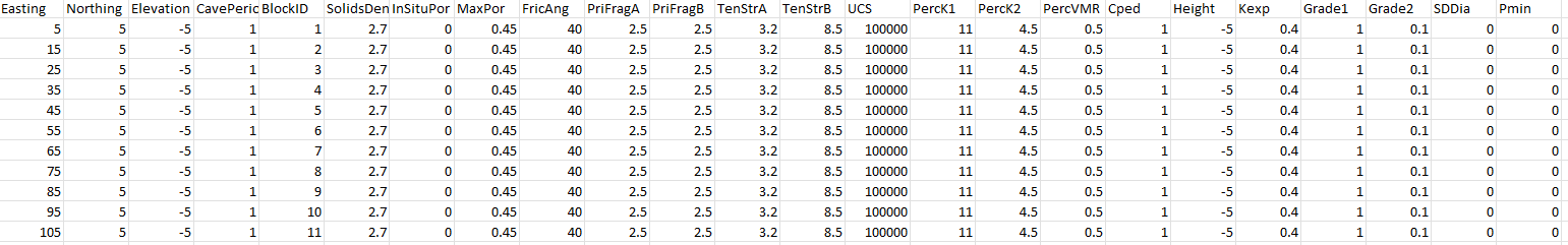
The required column names are: Easting, Northing, Elevation, CavePeriod, BlockID, SolidsDen, InSituPor, MaxPor, FricAng, PriFragA, PriFragB, TenStrA, TenStrB, UCS, PercK1, PercK2, and PercVMR ,in non-strict order but strict name. Additional columns are user-defined columns and often refer to ore graders (these are shown highlighted in yellow in the above figure). The labels for the ore grades come from the column headings. The file may contain any number (N) of ore grades.
Units: MassFlow assumes that all grades are provided as a percentage by mass and that friction angle is given in degrees. Any system of units may be used for the remaining quantities, but it is up to the user to ensure consistency among the various quantities (System of Units).
The succeeding lines of the data file are occupied by the block data. The number of blocks imported to MassFlow will have a direct impact on the memory requirements.
The properties required by the block model data file are described below:
Easting, Northing, Elevation — Position of the block center. All blocks must be aligned with the coordinate directions. The size of the block can be different in each of the coordinate directions (e.g., blocks 10 m x 15 m x 20 m are allowed), but all blocks must be the same size.
CavePeriod — The Period number in the draw schedule at which the block is capable of flowing. The block is made available for flow at the start of the specified Period. If a block is to be made available for flow from the start of the simulation, this number should be set to 1. If a block is never expected to flow (i.e., it lies outside the cave limits), CavePeriod should be set to a large number (larger than the number of Periods to be simulated). The choice of whether to specify cave limits in a simulation through the CavePeriod property depends on two factors: (1) whether cave stalling and associated free-surface development and rilling is to be simulated; and (2) whether cave stresses are of interest to the user. Cave stresses are calculated for reference only and, in Version 9.0, presently do not impact flow or fragmentation. (Note that stresses internal to the IMZ are estimated for secondary fragmentation calculations in Version 9.0, but these are independent of the cave stress calculations). If cave stalling is not to be simulated but cave stresses are of interest, the user should establish the lateral limits of the cave with the CavePeriod settings. If neither cave stalling nor cave stresses is of interest, the user is advised to set CavePeriod = 1 in all blocks.
Note: Initially CavePeriodDyn is assigned with this CavePeriod value. CavePeriodDyn is the dynamic version of the cave period, meaning that it can be changed by the user. By default, this is the same as CavePeriod. If it is different than CavePeriod (ifm, for example, it has been changed using FISH), then this value will be used instead of the value in CavePerdiod.
BlockID — A unique integer ID for the block. This is used for internal tracking and for reporting which blocks have material reporting to each drawpoint (see the section “Analyzing Results” for details on block-extraction reporting).
SolidsDen — Specific gravity (or true solids density) of the block material.
InSituPor — In-situ porosity of the block material. This is the porosity that the block material exhibits before it starts flowing. Porosity, \(n\), is related to the void volume, \(V_v\), and the total volume, \(V_t\), as follows: \(n = {{V_v}\over{V_t}}\) . It also is related to the in-situ density, InSituDen, and solids density, SolidsDen, as follows: \(n = 1 - SolidsDen/InSituDen\). Therefore, it should be set to zero in blocks that have not been caved. Blocks that lie within previously caved ground (e.g., in an overlying lift) are likely to have a porosity that is greater than zero (because it was previously flowing) but less than the maximum porosity inside the IMZs (MaxPor, described below), because some compaction likely will have occurred since it was caved.
MaxPor — Maximum porosity of the block material. This is the porosity that the block material exhibits once it has dilated fully (bulked) during flow (i.e., it is the porosity inside the IMZs. Porosity, \(n\), can be calculated as follows: \(n = B / (1 + B)\), where \(B\) is the bulking factor. The bulking factor is calculated by considering that an in-situ volume, \(V\), becomes a volume of \(V (1 + B)\) on bulking. The denominator in this equation \((1 + B)\) also is known as the swell factor, \(S\). MaxPor should not be estimated from the bulking factor, as it is calculated traditionally. This is because the bulking factor is calculated normally for the cave as a whole by combining estimates of the cave size with the mass drawn. A cave generally is comprised of both high-porosity flowing regions (IMZs) and lower-porosity stagnant regions. As a result, the bulking factor represents an average of these two and depends on the proportion of the cave that is flowing and stagnant. In MassFlow, the porosity of the stagnant regions is established by the InSituPor block property, and the porosity of the flowing regions is established with MaxPor block property. Depending on how cave draw is simulated in MassFlow, these two will combine to result in an overall cave porosity that is somewhere between InSituPor and MaxPor, and is more comparable to traditional bulking factors. (Note that there is presently no facility for calculating overall cave porosity or bulking factor in MassFlow, but this could be added in the future to permit comparison with mine-based bulking factor calculations.) Theoretically, MaxPor could be calculated by combining the estimate of IMZ size with the mass drawn from an isolated drawpoint. This is difficult (if not impossible) to achieve in practice, however; thus, it usually is estimated from the results of flow experiments or simulations. The results of such studies suggest that MaxPor is generally in the range 0.45-0.55.
FricAng — Friction angle of the block material. This is the friction angle that the caved rock exhibits inside the IMZ at its maximum porosity. FricAng controls three different behaviors in MassFlow: (1) the minimum angle that the base of the IMZ makes with the horizontal, calculated as \(45^{\circ} + FricAng/2\) (A large FricAng will result in a steep base to the IMZ.); (2) the angle of repose at the free surface, calculated as \(12^{\circ} + FricAng/2\) (A large FricAng will result in a steep angle of repose.); and (3) the stresses inside the IMZ, calculated in proportion to \(1/FricAng\). A large FricAng will result in lower stresses inside the IMZ. Theoretically, FricAng could be calculated by observing rill angles in the drawpoint, but this is difficult to achieve in practice. The results of shear box and triaxial tests conducted on a variety of different rock materials suggest that FricAng is generally in the range \(35-50^{\circ}\).
PriFragA - alpha value defining the shape of the Weibull distribution of primary fragmentation (see (20)).
PriFragB - beta value is the fragment size for the Weibull distribution of primary fragmentation. Initial fragment sizes are calculated according to (20).
An example is shown in Figure 5
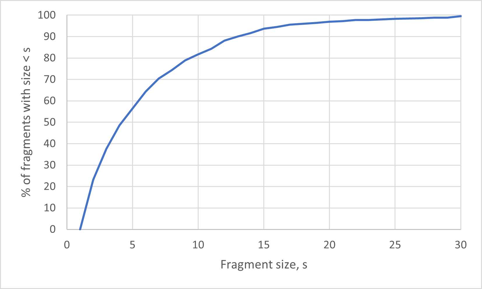
Figure 5: The cumulative size distribution for PriFragA = 0.86 and PriFragB = 0.45
Note: The attributes MeanDia, Mean diameter of the primary fragmentation expected in the block, and its dynamic version MeanDiaDyn for user-defined cahnges are computed as the Mean of a Weibull distribution following PriFragA and PriFragB. If MeanDiaDyn is different than MeanDia (ifm, for example, it has been changed using FISH), then this value will be used instead of the value in MeanDia. When a marker is created in MassFlow to track flow of caved material, it is assigned a fragment diameter that is sampled uniformly randomly from the Weibull distribution following PriFragA and PriFragB. Mean fragment diameter (calculated as the average by mass of all markers at a given level inside the IMZ) controls three main behaviors in MassFlow: (1) IMZ width, proportional to mean diameter inside the IMZ (A large mean diameter will result in a wider IMZ.); (2) the shear annulus at the periphery of the IMZ, which controls the internal velocity profile, always exhibiting a width that is 10 times the mean diameter (A large mean diameter will result in a more non-uniform velocity profile inside the IMZ.); and (3) rock-block strength, RBS, which is used for secondary fragmentation calculations, estimated from the user-defined core strength (UCS, described below) and the fragment diameter, \(d\), using the following relation of Hoek and Brown (1980): \(RBS = UCS(50/d)^{0.18}\). Larger fragments will exhibit a lower strength and a higher susceptibility to secondary fragmentation (rounding and splitting) inside the IMZ. The significance of these factors makes PriFragA and PriFragB one of the most important inputs to MassFlow.
TenStrA - alpha value defining the shape of the Weibull distribution of tensile strength.
TenStrB - beta value is the tensile strength (we estimate this from UCS or Is50) for the Weibull distribution of tensile strength.
UCS — Unconfined compressive strength of the intact block material. The UCS specified should correspond to that of a cylindrical core sample with a standard 5-cm diameter. The strength of the caved rock fragments is scaled from this value for secondary fragmentation calculations.
percK1 — Coefficient from the percolation rate equation below, used for local control of fines migration. Recommended base value k1=11. (This parameter is sensitive to strain rate. Note that there is a writing error in Pierce (2010) that erroneously attributes this sensitivity to k2 instead of k1.)
percK2 — Coefficient from the percolation rate equation below, used for local control of fines migration. Recommended base value k2=4.5
percVMR — Variance to mean ratio for percolation distance, used for local control of fines migration. During percolation event, equation below is used to estimate mean percolation distance L. VMR is used to establish random deviation from this mean, assuming Gaussian distribution. Standard deviation in perc distance is given by \(percSD=\sqrt {(VMR*L)}\). Recommended base VMR=0.5.
The percolation equation is given below:
Grade1….GradeN — Ore grade(s) of the block. A unique name can be specified in place of GradeN. The value is generally a percentage (0-100).
Draw Points
The drawpoint input file must be in the form of a comma-delimited table in csv. The file in input using the massflow drawpoint import command. As shown in the figure below, the first line contains the column headers. The columns must occur in the exact order shown. The succeeding lines of the data file are occupied by the drawpoint data. The exact strings used in the headers are not important but the order of the columns must be as depicted.
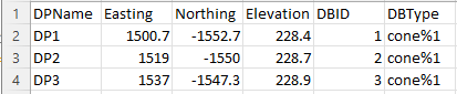
The properties required by the draw points data file are described below:
DPName — A unique name for the drawpoint. For SLC (Sub Level Caving) drawpoints, the end of the drawpoint name must contain the letter \(l\) followed by a number indicating the level on which the ring lies. Levels should increase in ascending numeric order with depth and must increment by 1 from level to level. This format is required for correct reporting of recoveries by origin and destination (i.e. primary, secondary etc.)
Easting, Northing, Elevation — Position of the drawpoint, which is defined as a point on the floor of the draw drift immediately below the brow (drawpoint drawbell or SLC ring), the center of the drawbell on the floor (drawpoint drawbell). All drawpoints must lie within the limits of the block model specified, but they do not need to be positioned relative to the blocks in any particular way. Drawpoints do not need to be at the same elevation.
Note that the location given in the file is at the bottom of the drift, but the draw actually occurs at the top of the drift. For rectangular drawbells, the draw occurs 1/2 drift width from the edges. See Figure 7
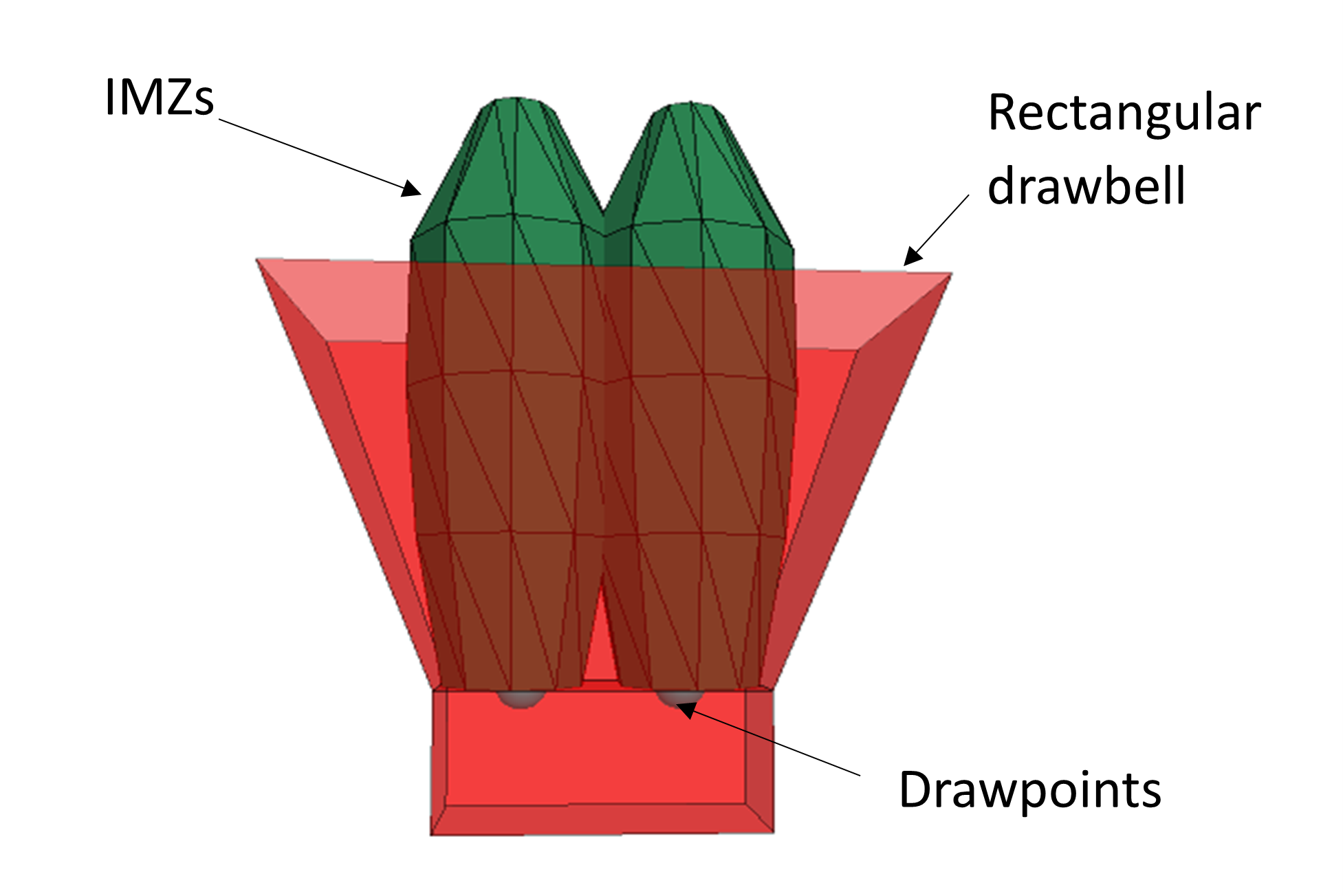
Figure 7: Location of draw and resulting IMZs for rectangular drawbells.
DBID — A unique number identifying the drawbell to which the drawpoint belongs. Two drawpoints will have the same DBID if they belong to the same drawbell.
DBType — A name that identifies the type of drawbell to which the drawpoint belongs. Two block caving drawpoints will have the same DBType if they belong to the same drawbell. Each drawbell can be of the same type or of a different type. The drawbell name must start with either “cone” (single drawpoint block caving drawbell), “rect” (two drawpoint block caving drawbell) or “slc” (sublevel caving ring), followed by the percent sign (%) and an id number. For example, slc%1 would specify one type of SLC ring that has a unique combination of ring dimensions, retreat azimuth and disturbed flow zone shape.
Draw Bells
Drawbell types must be imported into MassFlow using a separate input file. The file in input using the massflow drawbell import command. The input file must be in the form of a comma-delimited table in csv. As shown in the figure below, the first line contains the column headers. The columns must occur in the exact order shown. The succeeding lines of the data file are occupied by the drawbell properties discussed below.

There are three types of drawbells: conical, rectangular and SLC (Sub Level Caving). Each has a distinct set of properties necessary for definition, as shown below. In MassFlow Version 9, the only block caving (cone and rect) drawbell properties that affect IMZ growth and development are the draw-drift width and height. Future versions may restrict flow within the drawbell according to the specified geometry. In contrast, the SLC drawbell properties define the shape of the disturbed flow zone (which has a significant impact on the flow behavior), the ring geometry (which is needed for recovery tracking) and the retreat azimuth.
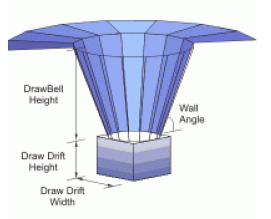
Figure 9: Conical drawbell geometry.
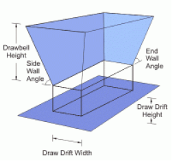
Figure 10: Rectangular drawbell geometry.
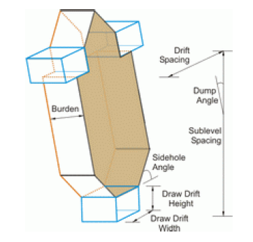
Figure 11: SLC drawbell geometry.
Properties for all drawbells
BellName - a unique identifier for the drawbell type. The drawbell name must start with either “cone” (single drawpoint block caving drawbell), “rect” (two drawpoint block caving drawbell) or “slc” (sublevel caving ring), followed by the percent sign (%) and an id number. For example, slc%1 would specify one type of SLC ring that has a unique combination of ring dimensions, retreat azimuth and disturbed flow zone shape.
DDWidth - the draw-drift width.
DDHeight - the draw-drift height.
Properties for conical and rectangular block caving drawbells (set to zero for SLC rings):
BellHeight - the drawbell height
SideAngle - the wall angle (conical) or sidewall angle (rectangular)
EndAngle - the end wall angle (rectangular) (not used for conical drawbells)
Note that for rectangular drawbells, the long horizontal dimension in Figure Figure #mass-rectangular is not defined in the drawbell geometry file. This dimension is calculated from the location of two drawpoints that make up the drawbell (see Figure 7).
Properties for SLC rings (set to zero for conical and rectangular drawbells):
DFZDepth - the depth of the Disturbed Flow Zone, measured horizontally from the blast ring across the burden.
DFZWidth - the width of the Disturbed Flow Zone, measured across the width of the ring, centered on crosscut drift.
DFZHeight - the height of the Disturbed Flow Zone, measured vertically upward from the brow.
SideHoleAngle - the angle that the ring sideholes make with the horizontal plane.
CrossCutSpacing - the horizontal distance between crosscuts, measured center to center.
SublevelSpacing - the vertical distance between sublevels, measured floor to floor.
Burden - the thickness of the ring, measured horizontally in the direction of the crosscut.
RetreatAz - the azimuth of retreat for the ring, measured clockwise from North.
The below figure illustrate the geometry of the DFZ and how height, width and depth are defined with respect to the ring.

Figure 12: Illustration of DFZ height, DFZ width, and DFZ depth.
Draw Schedule
DRAW SCHEDULE input files must be in the form of a comma-delimited table in csv. The file is input using the massflow drawpoint import-drawperiod command. As shown in the figure below, the first column contains the drawpoint names. Each succeeding column provides draw information for individual draw periods.
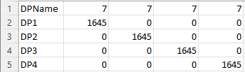
The length of the draw period and the period name are established by the column header. There are three different formats accepted for this header:
Integer — This number will be taken as both the period name and period length (in days).
String — The string will be taken as the period name, and the month name will be used to establish the period length in days (e.g., ‘Sept-08’ would result in a period length of 30 days).
PeriodName%PeriodLength — By using the separator character %, the user can specify both the period name and period length (in days) — e.g., Period1%20 would result in a period name of Period1 and a period length of 20 days.
Specifying Draw Masses
The numbers in each column represent the mass to be drawn from the corresponding drawpoint during that period. The mass units should be consistent with the units employed for the SolidsDen property in the block model file. MassFlow divides the total mass for the period by the period length to work out a daily tonnage. MassFlow updates marker locations on a daily basis; thus, the daily tonnage that results from this calculation should be within reason. If an unrealistically large draw mass is specified for a drawpoint marker (relative to the period length), updates will not be frequent enough to track material movements in the IMZ accurately.
Importing Multiple Draw Schedules
The user may import new draw periods at any time. When additional draw schedules are imported, MassFlow will delete any undrawn periods from the existing schedule and append the new draw periods. If an existing draw period is drawn only partially, it will be completed before the remaining (new) draw periods are drawn.
Model Outputs
Marker Report
By default, the format of the marker report is a tab-delimted text file as shown below
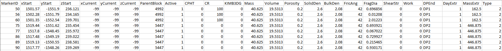
The file contains information about all markers. Extracted markers are listed first, followed by unextracted markers.
The columns are as follows:
MarkerID — ID of the marker.
xStart yStart zStart — Coordinates of the marker at the time it was created.
xCurrent yCurrent zCurrent — Current position of the marker. IF the marker has been extracted, these coordinates are -99
ParentBlock — ID of the parent mine block.
Active — Active state of the marker. Shows 1 if the marker has moved during the current period, otherwise shows 0.
Grade1….GradeN — User-defined data from the Mine Blocks. These headers can be any string and values can be any number. Often these are ore grades of the block with a value from 0-100.
Mass — Total mass associated with this marker.
Volume — Volume associated with this marker, where \(V = spacing^3/{1-\phi}\)
Porosity — Porosity associated with the marker, \(n\).
SolidDen — Density of host mine block, \(\rho\)
BulkDen — Bulk density of host mine block, where \(\rho_{bulk} = \rho*(1-\phi)\)
FricAng — Friction angle of the host mine block.
FragDia — Fragment diameter associated with the marker.
ShearStr — Shear strain associated with the marker.
Work — Work associated with the marker.
DPEnd — Drawpoint name. This value is “null” if the marker is not extracted.
DayExtr — Day of extraction. If not extracted, this value is -99.
MassExtr — Cumulative mass extracted. If not extracted, this value is -99 .
Type — Marker type. The types are as follows:
-2: unbulked for IMZ growth
-1: unbulked for collapse
0: unbulked for rilling
1: partially bulked
2: fully bulked
References
Cundall, P, Mukundakrishnan, B and Lorig, L 2000, REBOP (Rapid Emulator Based on PFC3D) formulation and user‘s guide, Itasca Consulting Group, Inc., Report to the International Caving Study, ICG00-099-7-20, October.
Laubscher, D 1994, Cave mining-the state of the art, Journal of the South African Institute of Mining and Metallurgy, pp. 279-293.
Nedderman, RM 1995, The use of the kinematic model to predict the development of the stagnant zone boundary in the batch discharge of a bunker, Chemical Engineering Science, vol. 50, pp. 959-965.
Pierce, M.E., 2010, A model for gravity flow if fragmented rock in block caving mines, PhD thesis, University of Queensland, Australia.
| Was this helpful? ... | Itasca Software © 2024, Itasca | Updated: Nov 12, 2025 |
