Linear Contact Model: Calibrating the Normal Critical Damping Ratio

Problem Statement

Note

The project file for this example may be viewed/run in PFC.[1] The data files used are shown at the end of this example.

When viscous damping is used in a PFC model with a linear contact model, an appropriate damping constant should be specified for the simulation to reproduce a realistic response. One way to do this is to calibrate the damping by using the relation between the damping constant and the restitution coefficient. [Kawaguchi1992] derived the relation by solving the equations of motion for free vibration with viscous damping. This derivation is presented. Also, the result of drop tests using PFC3D is compared with the analytical solution.

The linear contact model and its parameters are described in the “Linear Model” section.

The equation of motion for free vibration with viscous damping is given by Equation (1):

(1)\[m \ddot{x} + c\dot{x} + k x = 0\]

where \(m\) is the mass, \(c\) is the damping constant (coefficient of viscous damping), and \(k\) is the stiffness.

Solution of Equation (1) is given by Equation (2):

(2)\[x(t) = C_1 e^{(-\zeta+\sqrt{\zeta^2-1})^{\omega_n t}} + C_2 e^{(-\zeta-\sqrt{\zeta^2-1})^{\omega_n t}}\]

where \(C_1\) and \(C_2\) are arbitrary constants to be determined from the initial conditions. Also, \(\zeta\) is defined as the ratio of the damping constant to the critical damping constant, as given by Equation (3):

(3)\[\zeta = c / c_c\]

where \(c_c\) is the critical damping constant (Equation (4)):

(4)\[c_c = 2m\sqrt{\frac{k}{m}}=2 \sqrt{km} = 2 m \omega_n\]

where \(\omega_n\) is the natural frequency of the system.

This case corresponds to an underdamped system, as shown by the rebound of two impacting objects.

For the initial conditions \(x=x_0,\dot{x}(t=0)=\dot{x}_0\) , the solution for Equation (1) is given by Equation (5):

(5)\[x(t) = e^{-\zeta \omega_n t} \Big( x_0 \cos{\omega_d t} + \frac{\dot{x}_0 + \zeta \omega_n x_0}{\omega_d}\sin{\omega_d t} \Big)\]

where \(\omega_d\) is the frequency of the damped vibration, given by

(6)\[\omega_d = \sqrt{1-\zeta^2 \omega_n}\]

By substituting \(x-0\) = 0 into Equation (5):

(7)\[x(t) = e^{-\zeta \omega_n t} \Big( \frac{\dot{x}_0}{\omega_d}\sin{\omega_d t} \Big)\]

(8)\[\dot{x}(t) = -\zeta \omega_n e^{-\zeta \omega_n t} \Big( \frac{\dot{x}_0}{\omega_d}\sin{\omega_d t} \Big) + e^{-\zeta \omega_n t} \dot{x}_0 \cos{\omega_d t}\]

After half of the time period \(\pi/\omega_d\) (period of oscillation), the system recovers the position at \(x\) = 0. The velocity of the system is given by Equation (9):

(9)\[\dot{x}(t=\frac{\pi}{\omega_d}) = - e^{-\zeta \omega_n \frac{\pi}{\omega_d}} \dot{x}_0\]

Hence, the restitution coefficient \(\alpha\) is given by

(10)\[\alpha = - \frac{\dot{x}(t=\frac{\pi}{\omega_d})}{\dot{x}_0} = e^{-\zeta \omega_n \pi / \omega_d} = e^{-\frac{\zeta \pi}{\sqrt{1-\zeta^2}}}\]

Also, the ratio of the damping constant to the critical damping constant, \(\zeta\), and the damping constant, \(c\), are given by Equation (11) and Equation (12), respectively:

(11)\[\zeta = \frac{\ln(\alpha)}{\sqrt{\ln^2(\alpha)+\pi^2}}\]

(12)\[c = \frac{2\sqrt{km}\ln(\alpha)}{\sqrt{\ln^2(\alpha)+\pi^2}}\]

PFC3D model

A drop test is conducted in which two rows of 16 balls each are dropped under gravity from a one-meter height above a wall surface. The linear contact model is used, with a contact normal stiffness of \(k_n\) = 5.0 × 10⁴ and a change in the ratio of the damping constant to the critical damping constant (\(\beta_n\)) from 0.0 to 1.0. Also, the damping mode is set to \(M_d\) = 0 and \(M_d\) = 1. When \(M_d\) = 1, there is no tensile contact force between objects, and the critical damping ratio needs to be overestimated to achieve the same restitution coefficient.

The data file “restitution.dat (3D)” is used for this simulation, and the parameters of the simulation are summarized in the following table:

Table 1: Parameters of Simulation

Drop height	1 m
Ball diameter	50 mm
Ball density	2650 kg/m3
Contact normal stiffness (\(k_n\))	5 × 104 N/m
Contact shear stiffness (\(k_s\))	0
Friction coefficient (\(\mu\))	0
Normal critical damping ratio (\(\beta_n\))	0.0 to 1.0
Damping mode (\(M_d\))	0 and 1

The state of the system after solving for one second of mechanical time is shown in Fig. 1. Balls are contoured by their velocity magnitude. The critical damping ratio varies from 0.0 to 1.0 as \(x\) increases, hence the maximal rebound height for the balls close to \(x\) = 0.0, for which the collision is elastic. The contacts for the row of balls at \(y\) = 0.0 are set with \(M_d\) = 0, whereas the second row uses \(M_d\) = 1.

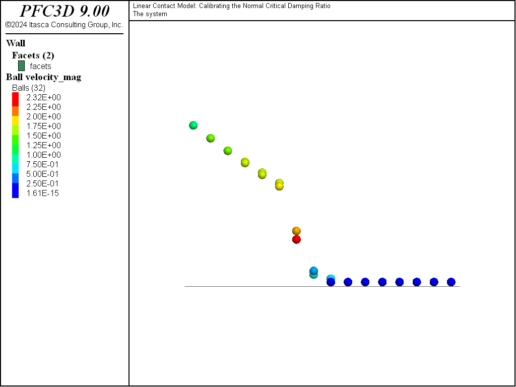
Figure 1: The system after one second of simulation.

Figures 2 and 3 show the \(z\)-position of the balls monitored during the simulation for \(M_d\) = 0 and \(M_d\) = 1, respectively, and illustrate the change in rebound height and frequency with \(\beta_n\) and \(M_d\).

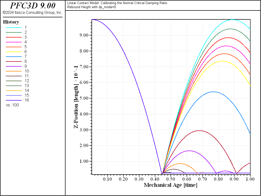
Figure 2: Ball z-position histories, \(M_d\) = 0.

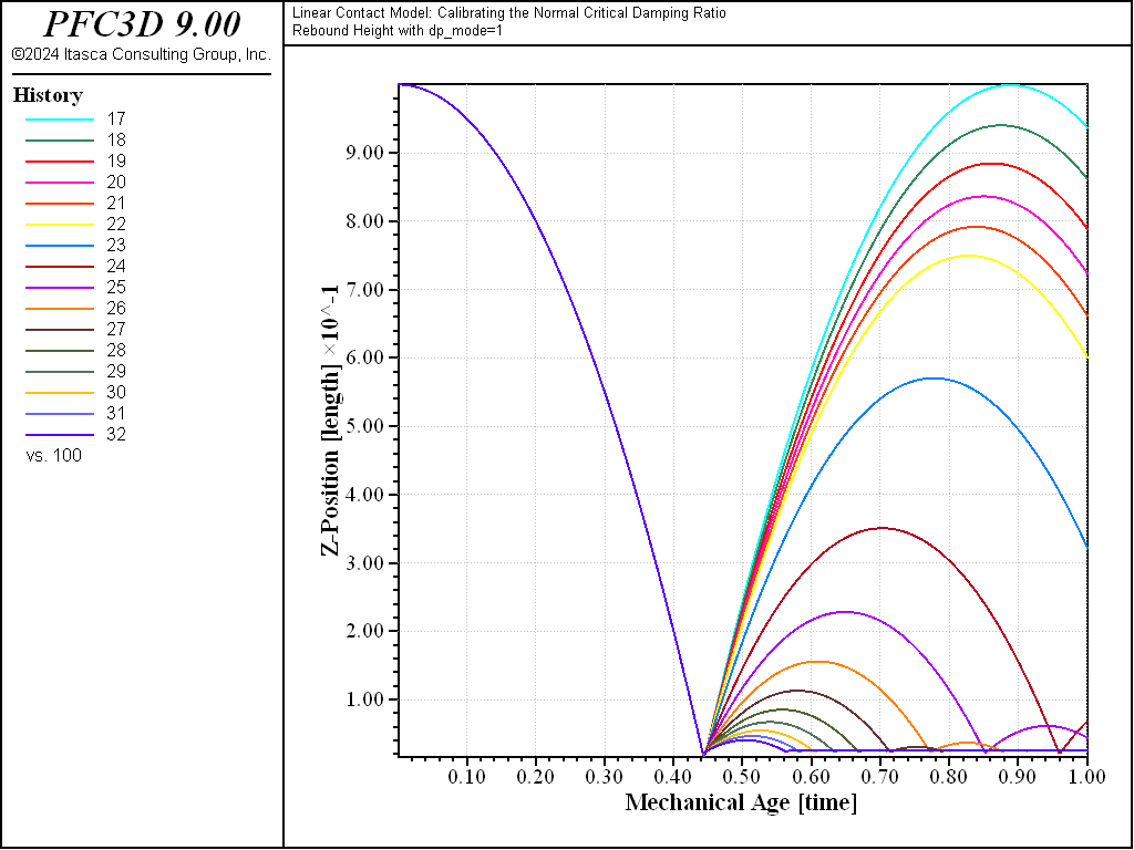
Figure 3: Ball z-position histories, \(M_d\) = 1.

The restitution coefficient is calculated from the maximum rebound height of the balls and plotted against the critical damping ratio for \(M_d\) = 0 (red marks) and \(M_d\) = 1 (green marks and dashed line) in Fig. 4, where the analytical solution given by Equation (10) is also reported (black dashed line). The maximum difference between the numerical and analytical solutions is less than 3%. Note that the accuracy of the numerical model depends on the time-integration granularity, both because the contact model implementation does and because the method chosen to evaluate the restitution coefficient in this example (measuring the rebound height) does. The results presented above are obtained with the timestep automatically evaluated by PFC. The simulation is repeated with a timestep fixed to a lower value (1 × 10^-5): the results (shown in Fig. 5) compare even better with the analytical solution (with a maximum difference less than 1%).

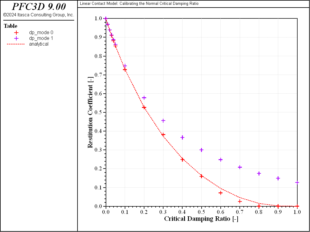
Figure 4: Relation between restitution coefficient and critical damping ratio.

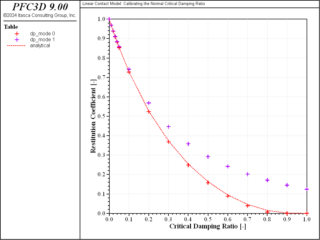
Figure 5: Relation between restitution coefficient and critical damping ratio. Simulation timestep fixed to 1 × 10^-5.

References

[Kawaguchi1992]

Kawaguchi, T. “Numerical Simulation of Fluidized Bed Using the Discrete Element Method (the Case of Spouting Bed),” in JSME (B), Vol. 58, No. 551, pp. 79-85 (1992).

Data Files

restitution.dat (3D)

; fname: restitution.p3dat
;
; Drop test under gravity: Exercise the linear contact model in the normal 
; direction with different values of the normal critical damping ratio and
; of the damping mode.
; Note the use of the Contact Model Assignment Table to assign different 
; contact model properties to every contact in this model, based on a spatial 
; range.
;
;=========================================================================
model new
model large-strain on
[global t1 = 'Linear Contact Model: ']
[global t2 = 'Calibrating the Normal Critical Damping Ratio']
model title [t1 + t2]

;-------------------------------------------------------------------------
; --------------------- Custom utility functions -------------------------
;-------------------------------------------------------------------------

fish define make_system(rad,height)
  local dia = 2.0*rad
  local _lx = 2*dia*16
  local _ly = 2*dia*2
  local _lz_inf = -0.5*dia
  local _lz_sup = height + 2.0*dia
  local _rad = 0.5*dia
  command
    model domain extent (0,[_lx]) (0,[_ly]) ([_lz_inf],[_lz_sup]) ...
           condition reflect reflect reflect
    wall generate id 1 polygon  0    0      0    ...
                                [_lx] 0      0    ...
                                0    [_ly]   0    ...   
                                [_lx] [_ly]   0 
    model history name '100' mechanical time-total  
    history interval 1
  end_command
  local _count = 0
  local _zpos = height
  local test = 1.0
  loop local j(1,2)
    local _ypos = dia *(2*j-1)
    local _ymin = _ypos - 0.5*dia
    local _ymax = _ypos + 0.5*dia
    loop local i(1,16)
      local _xpos = dia *(2*i-1)
      local _xmin = _xpos - 0.5*dia
      local _xmax = _xpos + 0.5*dia
      _count = _count+1
      command
        ball create id [_count] radius [rad] position [(_xpos,_ypos,_zpos)]
        ball history name [string(_count)] position-z id [_count]
      end_command
    end_loop
  end_loop
end

fish define fill_cmat(rad,kn)
  local _cn
  local _dpmode = 0
  loop local j(1,2)
    if j > 1 then
      _dpmode = 1
    endif
    local _ypos = 2.0*rad *(2*j-1)
    local _ymin = _ypos - rad
    local _ymax = _ypos + rad
    loop local i(1,16)
      local _xpos = 2.0*rad *(2*i-1)
      local _xmin = _xpos - rad
      local _xmax = _xpos + rad
      if i <= 6 then
        _cn = 0.0 + (i-1.0)*0.01
      else
        _cn = 0.0 + (i-6)*0.1
      endif
      command
        contact cmat add model linear ...
              property kn [kn] dp_nratio [_cn] dp_mode [_dpmode] ...
              range position-x [_xmin] [_xmax] ...
              position-y [_ymin] [_ymax]
      end_command
    end_loop
  endloop
end

fish define make_tables(rad,height) 
    global get_hist_max
    local tab_ana = table.create('analytical')
    local tab_dp0 = table.create('dp_mode 0')
    local tab_dp1 = table.create('dp_mode 1')
    tab_dp = tab_dp0
    loop local j(1,2)
        local histfirst = 1 + 16*(j-1)
        loop local i(1,16)
            local _cn
            if i <= 6 then
                _cn = 0.0 + (i-1)*0.01
            else
                _cn = 0.0 + (i-6)*0.1
            endif    
            if j = 1 then
                local rth
                if _cn # 1.0 then
                    rth = -1.0 *_cn * math.pi / math.sqrt(1.0-_cn*_cn)
                    rth = math.exp(rth)
                else
                    rth = 0
                endif
                table.value(tab_ana,i) = vector(_cn,rth)
            endif
            local hid = histfirst + (i-1)
            local reb_h = get_hist_max(hid) - rad 
            reb_h = math.max(reb_h,0.0)
            local repu = math.sqrt(reb_h /(height-rad))
            table.value(tab_dp,i) = vector(_cn,repu)
        endloop
        tab_dp = tab_dp1
    endloop
    global err = 0
    loop i (1,16)
        err = math.max(err,math.abs(table.y(tab_dp0,i)-table.y(tab_ana,i)))
    endloop
end

fish define get_hist_max(hid)
  ; get the first maximum of a history 
  tab_tmp = table.create('dummy')
  command
    history export [string(hid)] table 'dummy'
  endcommand
  ; pass first minimum, then find first maximum (height of rebound)
  local tsize = table.size(tab_tmp)
  local minpassed = 0
  local max_h = -1e20
  section
    loop local it(2,tsize)
      local _y1 = table.y(tab_tmp,it-1)
      local _y2 = table.y(tab_tmp,it)
      if minpassed = 0 then
        if _y2 > _y1 then
          minpassed = 1
        endif
      else
        max_h = math.max(max_h,_y2)
        if _y2 < max_h then
          exit section
        endif
      endif  
    endloop
  end_section
  table.delete(tab_tmp)
  get_hist_max = max_h
end

;-------------------------------------------------------------------------
; ---------------------------- SIMULATION --------------------------------
;-------------------------------------------------------------------------

[global ball_radius=0.025]
[global drop_height=1.0]

[make_system(ball_radius,drop_height)]
[fill_cmat(ball_radius,5.0e4)]
ball attribute density 2650
model gravity 0 0 -10.0
model save 'ini'
model solve age 1.0
;
[make_tables(ball_radius,drop_height)]
model save 'final'

model restore 'ini'
model mechanical timestep fix 1e-5
model solve age 1.0
;
[make_tables(ball_radius,drop_height)]
model save 'final-dtfix'

program return 
;=========================================================================
; eof: restitution.p3dat

Endnote

[1]

This example is listed under the present document title in the i Examples dialog (use the menu command Help -> Examples… to access).