Examples • Example Applications

Fluid Flow Towards a Tunnel (FLAC2D)

Problem Statement

Note

This project reproduces Example 1.3 from the FLAC 8.1 fluid flow manual. The project file for this example is available to be viewed/run in FLAC2D. The project’s main data files are shown at the end of this example.

This example analyzes the steady-state flow toward a tunnel encircled by a ring of material (for example, as produced by grouting) that has one-tenth the permeability of the surrounding material. There is also a high-permeability layer at the ground surface that consists of material with ten times the permeability of the rest of the model. The problem illustrates the benefit of using the steady-state solver for fluid analysis. The effectiveness of the implicit versus the explicit solver is also explored.

Model Geometry

For this model, half symmetry is assumed. The model is constructed in Sketch as follows:

1. Use the Corner,Corner tool and draw a box from 0,0 to 80,20.

2. Draw a horizontal line from 0,17 to 80,17

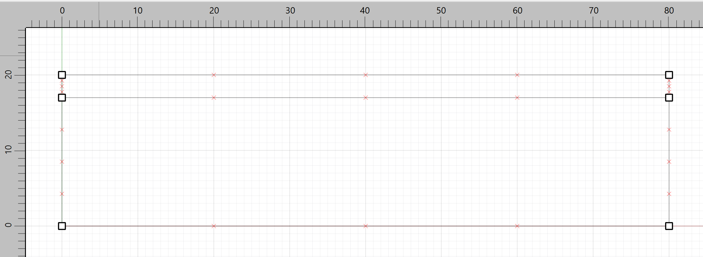
3. Draw a circle using the Diameter option. Click points at 0,1 and 0,15

4. Select the point outside of the rectangle and delete it.

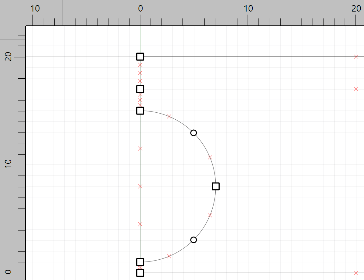
5. Repeat to draw a half a circle with points 0,4 and 0,12

6. Set the zone size to 1. Select Set meshing parameters from the zoning menu and check the box for Create unstructred meshes only, the click the button the Mesh Now. (If a strutured mesh is allowed then the inner circle produces very thin zones around the edges.)

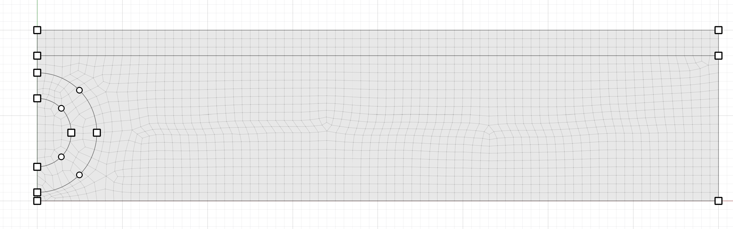
7. Set group names for the zones as shown below.

8. Finally, select the two edges that define the tunnel surface and assign them them group name “tunnel wall”.

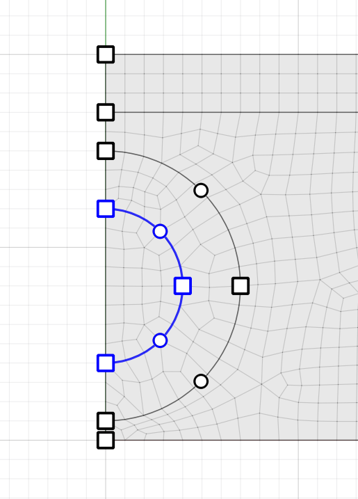
9. Create the zones, save the project and the model state. The rest of the model is developed using commands in a data file as shown at the end of this example.

Model Solution

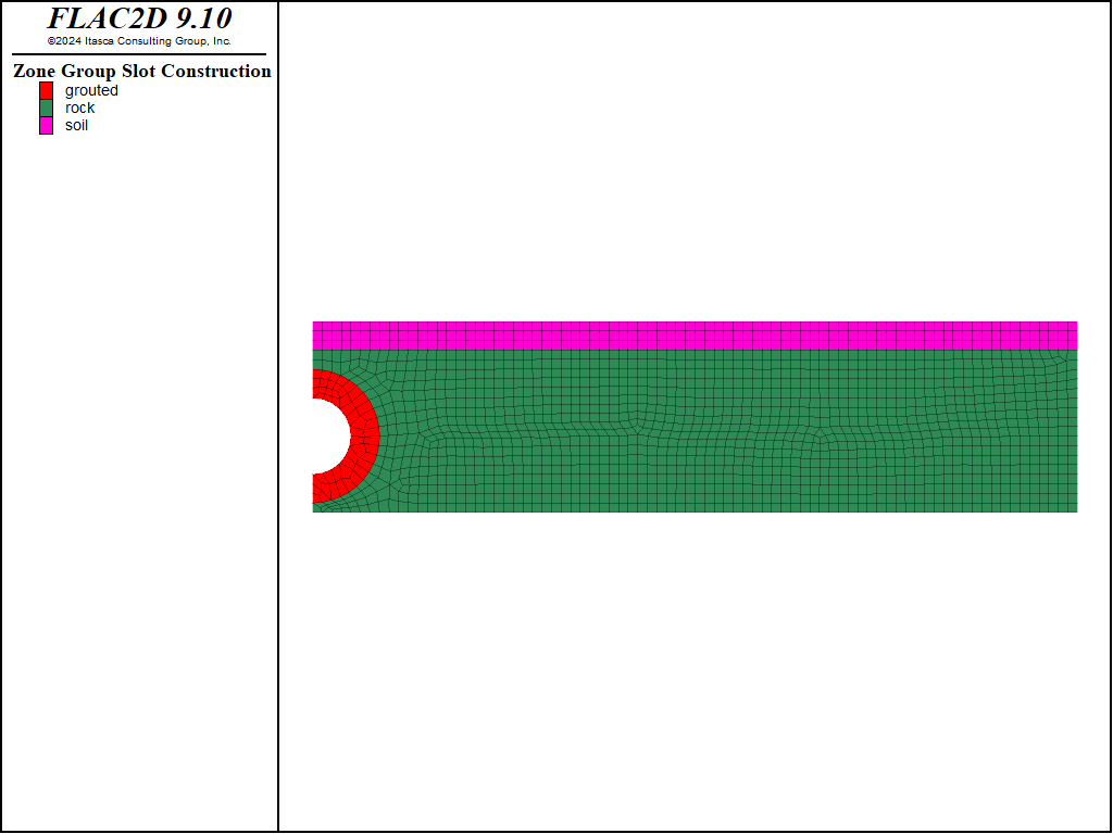
Figure 6 shows the various regions in the model. A hydrostatic pressure is imposed on the right-hand boundary, and the tunnel pressure is maintained at zero. The cutoff model is used to simulate unsaturated flow and a phreatic surface develops in the model.

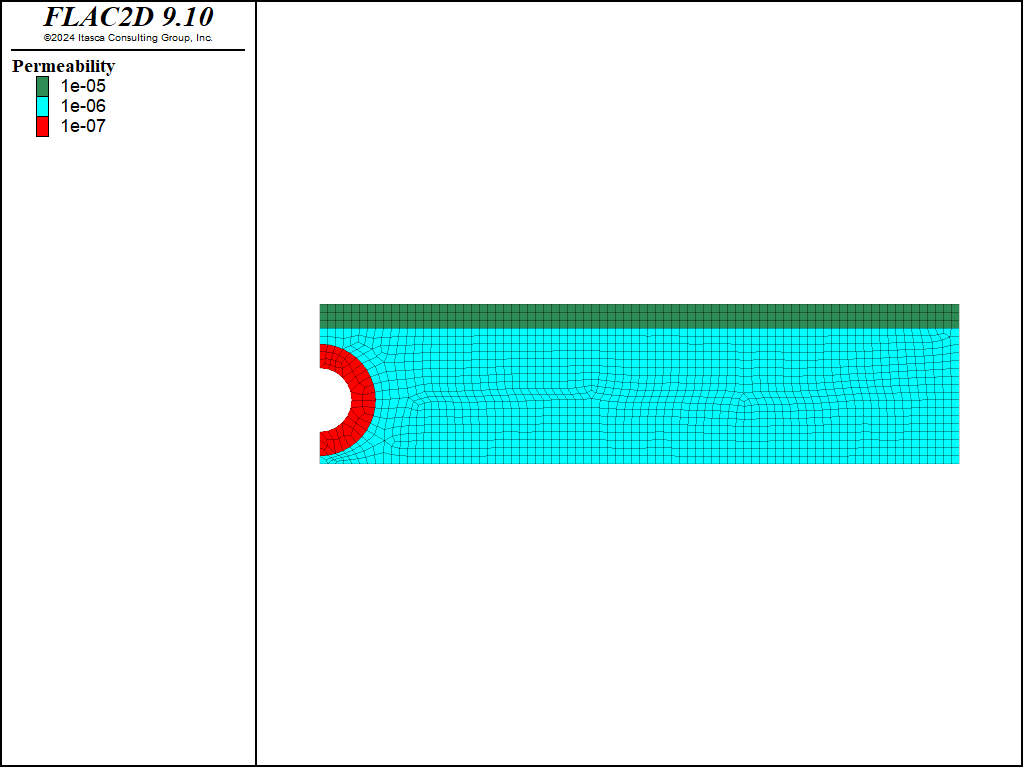
Figure 6: Material permeabilities in the tunnel model.

The command zone fluid steady-state can be used to solve to steady state pore pressures in one step. This command does not do any calculation steps and solves the problem more or less instantaneously. The resulting pore pressures for the steady state ananlysis are shown in Figure 7. Note that the solution does not converge for the default number of iterations (300). The resulting solution is quite close to reaching the default tolerance (1e-5), but if a more accurate answer is required, increase the number of iterations as shown in this example.

Figure 7: Steady-state pore pressures in the model.

The same model could be solved by time stepping using an explicit or implicit approach. A FISH function can be used to monitor how close you are to steady state. When boundary nodes have a fixed pore pressure, a FISH function can be used to to measure total flow (in volume/time units) into the grid (sum of positive flows) and total flow out of the grid (sum of negative flows). The FISH function shown below computes inflow and outflow, and histories of these variables can be taken to monitor the evolution towards steady state. This function also computes qratio, which is the absolute difference in inflow and outflow values, divided by their mean. The value of qratio is a dimensionless number that may be used in a test for convergence. It is equivalent to the built-in ratio calculated when solving fluid flow problems.

The model is run in implicit model using the built-in servo to automatically determine the optimum timestep. Note that the servo functionality may also turn off the implicit logic (and revert to explicit) if the error is becoming too large (see zone fluid implicit servo). If the default error threshold is used (1e-8), then you will see the model flipping back and forth from implicit to explicit. This will work, but you can reach the solution faster by reducing the error threshold that is used to determine when to switch back to explicit. In this example, an error threshold of 1e-5 is used.

For rapid solution to steady state, the fluid bulk modulus is set using equation 12 of the fluid manual (time-scales). If the actual time evolution of pore pressures is important, and a fluid-only analysis is being performed, the command zone fluid modulus-scale can be used to set the fluid modulus to give the correct time response. In this case the user must first set the mechanical stiffnesses and true fluid bulk modulus. If a coupled analysis is being performed (mechanical and fluid), the the command zone fluid modulus-automatic should be used.

The histories of inflow and outflow for the implicit solution are plotted in Figure 8. It can be seen that the inflow and outflow converge towards one another. As mentioned above, the flow time is not realistic. Figure 9 shows contours of pore pressure at a ratio of 0.01 (assumed to be close to steady state); the phreatic surface exhibits discontinuities in slope where it crosses the permeability contrasts. This is very similar to the steady state solution above, the main difference being the length of calculation time required.

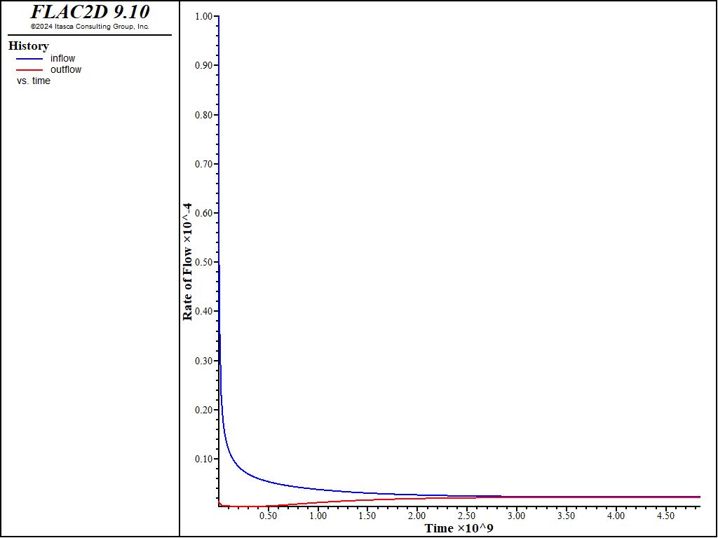
Figure 8: Histories of inflow and outflow for the implicit solution.

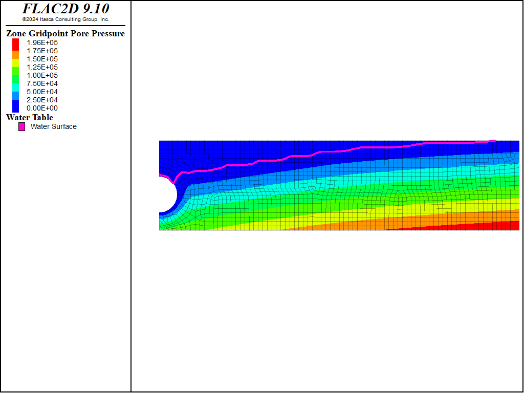
Figure 9: Pore pressure contours for the implicit solution.

Results for the explicit solution are shown in Figure 10 and Figure 11. Results are similar to the implicit solution. The main difference is that it took approximately 5x longer to reach the solution in this case.

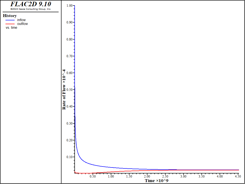
Figure 10: Histories of inflow and outflow for the explicit solution.

Figure 11: Pore pressure contours for the explicit solution.

Data Files

ShallowTunnel.dat

;Based on FLAC 8.1 steady state example (Shallow Tunnel)

model new
model restore 'sketch'
zone face skin

model configure fluid-flow

model gravity 9.81

zone fluid-density 1000
zone fluid property porosity 0.5

; civil engineering permeability (m/s)
zone fluid property hydraulic-conductivity 1.0e-6
zone fluid property hydraulic-conductivity 1.0e-5  range group 'soil'
zone fluid property hydraulic-conductivity 1.0e-7 range group 'grouted'

zone face apply head 20 range group 'East'

zone fluid unsaturated cutoff 
zone face apply pore-pressure 0 range group 'Top'

zone delete range group 'tunnel'

zone face apply pore-pressure 0 range group 'tunnel wall'

model save 'fluid-initial'

zone fluid steady-state
model save 'fluid-steady'

implicit.dat

; test - implicit
model restore 'fluid-initial'

program call 'qratio.fis'

fish history name 'ratio' qratio 
fish history name 'inflow' inflow 
fish history name 'outflow' outflow 
model history name 'time' fluid time-total

zone nodal-mixed-discretization off
zone fluid property fluid-modulus [0.3*1*1000*10/0.5]  ; eq 12
zone fluid implicit servo on 
model solve-fluid ratio-flow 0.01
model save 'fluid-implicit'

explicit.dat

; test - explicit
model restore 'fluid-initial'

program call 'qratio.fis'

fish history name 'ratio' qratio 
fish history name 'inflow' inflow 
fish history name 'outflow' outflow 
model history name 'time' fluid time-total

zone nodal-mixed-discretization off
zone fluid property fluid-modulus [0.3*1*1000*10/0.5]  ; eq 12
model solve-fluid ratio-flow 0.01
model save 'fluid-explicit'

qratio.fis

fish define qratio
  global inflow = 0.0
  global outflow = 0.0
  loop foreach local gp gp.list
    if gp.pp.fix(gp)
      if gp.flow(gp) > 0
        inflow += gp.flow(gp)
      else
        outflow -= gp.flow(gp)
      end_if
    end_if
  end_loop
  local qbalance = inflow - outflow
  if (inflow + outflow) # 0
    qratio = 2.0*math.abs(qbalance)/(inflow+outflow)
  else
    qratio = 0.0
  end_if
end