Replicating a Particle Size Distribution
Introduction
Note
The project file for this example may be viewed/run in PFC.[1] The data files used are shown at the end of this example.
This example involves the creation of a particle assembly starting from a Particle Size Distribution (PSD) curve. The entire procedure, from sieve analysis data to ball assembly, is presented.
Numerical Model
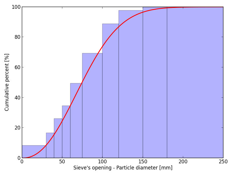
Sieve analysis is a technique commonly used to measure the gradation in particle size of a granular material. The test usually consists of shaking aggregate in nested sieves with progressively smaller mesh sizes. The table below presents the result of a sieve analysis applied to a crushed sample of limestone. The mass percentage of material within each size range is shown.
0 - 30 |
8.3 |
|
30 - 40 |
8.3 |
|
40 - 50 |
9.4 |
|
50 - 60 |
8.5 |
|
60 - 75 |
14.8 |
|
75 - 100 |
20.0 |
|
100 - 120 |
19.5 |
|
120 - 150 |
8.8 |
|
150 - 180 |
2.1 |
|
180 - 250 |
0.3 |
A Rosin-Rammler curve (see Equation (1)) can be used to describe the cumulative PSD curve associated with the data of Table 1:
where \(D_{pRR}\) and \(n_{RR}\) are two parameters that determine the position and shape of the curve. We use \(D_{pRR}\)=0.0876 and \(n_{RR}\)=2.25 for this example.

Figure 1: Mass percentages of retained particles (blue bars) along with the cumulative mass percentage (Rosin-Rammler curve; red dotted line).
The lines contained in the file granulometry.dat (3D) are presented below. The random seed is set so that the results will be exactly reproducible. A table containing the data from the sieve analysis (i.e., the data in Table 1) is created with FISH.
A second table, containing values that are used to draw the Rosin-Rammler curve to compare with the PFC model, is also created. This step is for comparative purposes and is not required.
A domain must be created prior to the instantiation of balls. The ball distribute command is used, along with the data in Table 1, to create the specimen. Balls are placed inside a box to match a target porosity and size distribution without regard to overlap. Ten bins are defined based on a range of radii and volume fractions. Note the use of the model random command to set the seed of the pseudo-random number generator, thus ensuring reproducibility of the model. This command may be omitted, or the seed changed to a different integer number, to produce different configurations.
To verify the accuracy of the result, one may use the measure create command to create a measurement sphere, specifying the number of bins for the size distribution calculation with the bin keyword. All balls that fall within the measurement region are binned based on their diameters. The cumulative volume percentage (between 0 and 1) of balls as a function of bin size is calculated and exported to a table with the measure dump command.
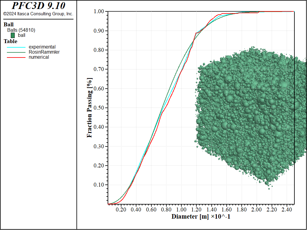
The table named numerical is used as the basis to plot the size distribution of the sample that has been generated. A direct comparison with the Rosin-Rammler curve is possible (Figure Figure #tut-gran-comparison). The comparison demonstrates that the ball distribute command is capable of reproducing sieve analysis results. Note that the Rosin-Rammler curve has been artificially built on the base of the raw data coming from the sieve analysis. The numerical result would be closer to this curve if a higher number of bins were employed in the ball distribute command.

Figure 2: Comparison between the input PSD curve (Rosin-Rammler - green), the experimental curve from Table 1 (blue), and the PSD curve obtained from the measure logic in PFC (red).
Discussion
This tutorial presents the steps required to produce a model consisting of overlapping balls where the balls follow a realistic particle size distribution resulting from a sieve analysis. The balls have been generated in a box so that the cumulative sum of the ball volumes is a specified fraction of the box volume. These exact steps could be followed with clumps using the clump distribute command. One should be aware, though, that the resulting porosity of the specimen after equilibration will not be identical to the specified porosity. This is due to the fact that balls will overlap in the equilibrated system. If the ball overlaps are small, then the difference may be negligible.
Data Files
granulometry.dat (3D)
; fname: Granulometry.dat (3D)
;
;  Create a balls assembly from a Particle Size Distribution of a limestone
;  sample
;=========================================================================
model new

;Input raw data of limestone granulometry
fish define granulometry
  global exptab = table.create('experimental')
  table(exptab,0.03) = 0.083
  table(exptab,0.04) = 0.166
  table(exptab,0.05) = 0.26
  table(exptab,0.06) = 0.345
  table(exptab,0.075) = 0.493
  table(exptab,0.1) = 0.693
  table(exptab,0.12) = 0.888
  table(exptab,0.15) = 0.976
  table(exptab,0.18) = 0.997
  table(exptab,0.25) = 1.0
end
[granulometry]

fish define RosinRammler(Dp_rr,n_rr,dmin)
  global t = "RosinRammler"
  loop local i (1,1000)
    freq = math.random.uniform
    temp = Dp_rr*((-math.ln(1-freq))^(1/n_rr))
    table(t,temp)=freq
  endloop
end
[RosinRammler(0.0876,2.25,0.002)]

; Generate the sample
[global domain_extent = 1.0]
model domain extent [-domain_extent] [domain_extent]
[global dmin = 0.001]

model random 10001
ball distribute box ([-domain_extent*0.7],[domain_extent*0.7])        ...
        porosity 0.36                                                 ...
        number-bins 10                                                ...
        bin 1                                                         ...
            radius [0.5*dmin] [0.5*table.x(exptab,1)]                 ...
            volume-fraction [table.y(exptab,1)]                       ...
        bin 2                                                         ...
            radius [0.5*table.x(exptab,1)] [0.5*table.x(exptab,2)]    ...
            volume-fraction [table.y(exptab,2)-table.y(exptab,1)]     ...
        bin 3                                                         ...
            radius [0.5*table.x(exptab,2)] [0.5*table.x(exptab,3)]    ...
            volume-fraction [table.y(exptab,3)-table.y(exptab,2)]     ...
        bin 4                                                         ...
            radius [0.5*table.x(exptab,3)] [0.5*table.x(exptab,4)]    ...
            volume-fraction [table.y(exptab,4)-table.y(exptab,3)]     ...
        bin 5                                                         ...
            radius [0.5*table.x(exptab,4)] [0.5*table.x(exptab,5)]    ...
            volume-fraction [table.y(exptab,5)-table.y(exptab,4)]     ...
        bin 6                                                         ...
            radius [0.5*table.x(exptab,5)] [0.5*table.x(exptab,6)]    ...
            volume-fraction [table.y(exptab,6)-table.y(exptab,5)]     ...
        bin 7                                                         ...
            radius [0.5*table.x(exptab,6)] [0.5*table.x(exptab,7)]    ...
            volume-fraction [table.y(exptab,7)-table.y(exptab,6)]     ...
        bin 8                                                         ...
            radius [0.5*table.x(exptab,7)] [0.5*table.x(exptab,8)]    ...
            volume-fraction [table.y(exptab,8)-table.y(exptab,7)]     ...
        bin 9                                                         ...
            radius [0.5*table.x(exptab,8)] [0.5*table.x(exptab,9)]    ...
            volume-fraction [table.y(exptab,9)-table.y(exptab,8)]     ...
        bin 10                                                        ...
            radius [0.5*table.x(exptab,9)] [0.5*table.x(exptab,10)]   ...
            volume-fraction [table.y(exptab,10)-table.y(exptab,9)]

measure create id 1 radius [domain_extent*0.6] ...
                    bins 100 [dmin] [table.x(exptab,10)]
measure dump id 1 table 'numerical'

program return
;=========================================================================
; eof: Granulometry.dat (3D)
Endnote
| Was this helpful? ... | Itasca Software © 2024, Itasca | Updated: Aug 13, 2024 |
