FLAC3D Theory and Background • Interfaces
Choice of Material Properties
Assignment of material properties (particularly stiffnesses) to an interface depends on the way the interface is used. Three possibilities are common. The interface may be:
an artificial device to connect two sub-grids together;
a real interface that is stiff compared to the surrounding material, but which can slip and perhaps open in response to the anticipated loading. (This case also encompasses the situation in which stiffnesses are unknown or unimportant, but where slip and/or separation will occur, e.g., flow of frictional material in a bin.); or
a real interface that is soft enough to influence the behavior of the system (e.g., a joint with soft clay filling or a dike containing heavily fractured material).
These cases are examined in detail.
Interface Used to Join Two Sub-grids
If possible, sub-grids should be joined with the zone attach command.
It is more computationally efficient to use the zone attach command than the
zone interface create command to join sub-grids. See Connecting Adjoining Primitive Shapes
for a description of, and restrictions on, the zone attach command.
Under some circumstances, it may be necessary to use an interface to join two sub-grids.
This type of interface is assigned high strength properties with the
zone interface node property command, thus preventing any slip or separation. (This is
the equivalent of a “glued” interface in FLAC.) Shear and normal stiffnesses must also be
provided; values of friction and cohesion are not needed. It is tempting (particularly for
people familiar with finite element methods) to give a very high value for these stiffnesses to
prevent movement on the interface. However, FLAC3D does “mass scaling” (see
Mechanical Timestep Determination for Numerical Stability) based on stiffnesses, and the response (and solution
convergence) will be very slow if very high stiffnesses are specified. It is recommended that
the lowest stiffness consistent with small interface deformation be used. A good rule-of-thumb
is that \(k_n\) and \(k_s\) be set to ten times the equivalent stiffness of the
stiffest neighboring zone. The apparent stiffness (expressed in stress-per-distance units) of a
zone in the normal direction is
where:
\(K\) & \(G\) are the bulk and shear moduli, respectively; and
\(\Delta z_{\min}\) is the smallest width of an adjoining zone in the normal direction (see Figure 1).
The \(\max\) [ ] notation indicates that the maximum value over all zones adjacent to the interface is to be used (e.g., there may be several materials adjoining the interface).
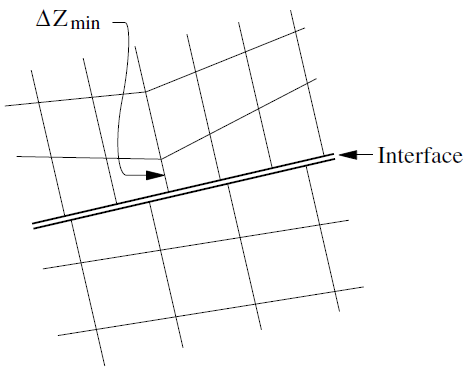
Figure 1: Zone dimension used in stiffness calculation.
To illustrate the approach, consider Figure 2, in which two sub-grids of unequal zoning are joined by the commands in “Subgrids.dat”, and are loaded by a pressure on the left-hand part of the upper surface. To view this project, use the menu command . This is the the “Subgrids.prj” project.
Subgrids.dat
model new
model large-strain off
model title "Joining two sub-grids"
fish automatic-create off
zone create brick size 4 4 4 point 0 (0,0,0) point 1 (4,0,0) ...
                             point 2 (0,4,0) point 3 (0,0,2)
zone create brick size 8 8 4 point 0 (0,0,3) point 1 (4,0,3) ...
                             point 2 (0,4,3) point 3 (0,0,5)
zone interface 'joint' create by-face range position-z 3
zone interface node property stiffness-normal 300e9 ...
                             stiffness-shear 300e9 ...
                             tension 1e10 ...
                             shear-bond-ratio=1
zone gridpoint initialize position-z -1.0 add range position-z 3 5
zone cmodel assign elastic
zone property bulk 8e9 shear 5e9
zone gridpoint fix velocity-z range position-z 0
zone gridpoint fix velocity-x range union position-x 0 position-x 4
zone gridpoint fix velocity-y range union position-y 0 position-y 4
zone face apply stress-zz -1e6 ...
                range position-z 4 position-x 0,2 position-y 0,2
model solve
model save 'join.f3sav'
The value of \((K+4G/3)\) is 15 GPa, and the minimum zone size adjacent to the interface is 0.5 m. Hence, we choose both shear stiffness and normal stiffness to be 150 × 109/0.5 (i.e., \(k_n = k_s = 3 \times 10^{11}\) Pa/m). The resulting contours of \(z\)-displacement are shown in Figure 3.
Compare this result to that for a single grid shown in this figure. This plot is at the same scale and contour intervals as Figure 3. The two plots are almost identical, which indicates that the interface does not affect the behavior to any great extent.
The prescription given in Equation (1) is reasonable if the materials on the two sides of the interface are similar and variations of stiffness occur only in the lateral directions. However, if the material on one side of the interface is much stiffer than that on the other, then Equation (1) should be applied to the softer side. In this case, the deformability of the whole system is dominated by the soft side; making the interface stiffness ten times the soft-side stiffness will ensure that the interface has minimal influence on system compliance.
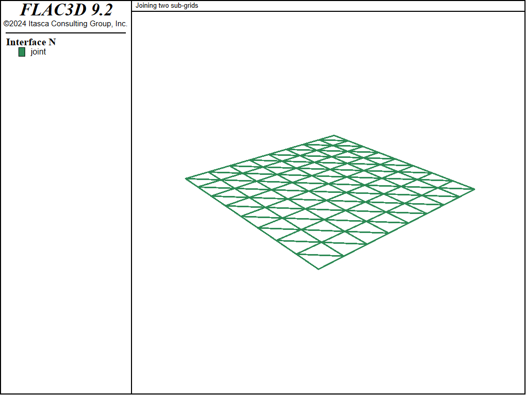
Figure 2: Two unequal sub-grids joined by an interface.
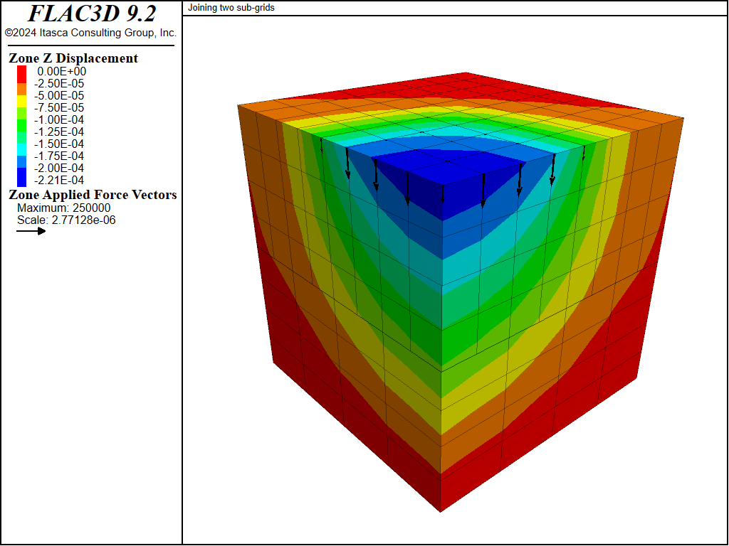
Figure 3: Vertical displacement contours—two joined grids.
Real Interface — Slip and Separation Only
In this case, we simply need to provide a means for one sub-grid to slide and/or open relative to another sub-grid. The friction (and perhaps cohesion, dilation, and tensile strength) is important, but the elastic stiffness is not. The approach in Interface Used to Join Two Sub-grids is used here to determine \(k_n\) and \(k_s\). However, the other material properties are given real values (for advice see All Properties Have Physical Significance).
As an example, we can allow slip in a bin-flow problem, as shown in Figure 4, corresponding to the data file in “BinFlowSlip.dat”. To view this project, use the menu command . This is the the “BinFlowSlip.prj” project. The bond strengths are not set (i.e., they default to zero); the interface stiffnesses are set to approximately ten times the equivalent stiffness of the neighboring zones.
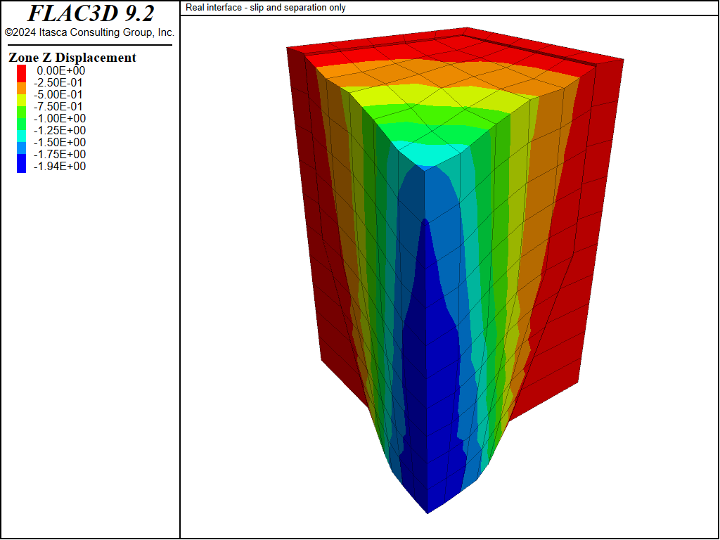
Figure 4: Flow of frictional material in a “bin”.
BinFlowSlip.dat
model new
model title "Real interface - slip and separation only"
fish automatic-create off
; Create Material Zones
zone create brick size 5 5 5 ...
         point 0 (0,0,0) point 1 (3,0,0) point 2 (0,3,0) point 3 (0,0,5) ...
         point 4 (3,3,0) point 5 (0,5,5) point 6 (5,0,5) point 7 (5,5,5)
zone create brick size 5 5 5 point 0 (0,0,5) edge 5.0
zone group 'Material'
; Create Bin Zones
zone create brick size 1 5 5 ...
         point 0 (3,0,0) point 1 add (3,0,0) point 2 add (0,3,0) ...
         point 3 add (2,0,5) point 4 add (3,6,0) point 5 add (2,5,5) ...
         point 6 add (3,0,5) point 7 add (3,6,5) group 'Bin1'
zone create brick size 1 5 5 ...
         point 0 (5,0,5) point 1 add (1,0,0) point 2 add (0,5,0) ...
         point 3 add (0,0,5) point 4 add (1,6,0) point 5 add (0,5,5) ...
         point 6 add (1,0,5) point 7 add (1,6,5) group 'Bin1'
zone create brick size 5 1 5 ...
         point 0 (0,3,0) point 1 add (3,0,0) point 2 add (0,3,0) ...
         point 3 add (0,2,5) point 4 add (6,3,0) point 5 add (0,3,5) ...
         point 6 add (5,2,5) point 7 add (6,3,5) group 'Bin2'
zone create brick size 5 1 5 ...
         point 0 (0,5,5) point 1 add (5,0,0) point 2 add (0,1,0) ...
         point 3 add (0,0,5) point 4 add (6,1,0) point 5 add (0,1,5) ...
         point 6 add (5,0,5) point 7 add (6,1,5) group 'Bin2'
; Assign models to groups
zone cmodel assign mohr-coulomb range group 'Material'
zone cmodel assign elastic range group 'Bin1' or 'Bin2' or 'Bin3' or 'Bin4'
; Separate zones, and create two interfaces
zone separate by-face new-side group 'Interface' ...
                      range group 'Material' group 'Bin1' or 'Bin2'
zone interface create by-face range group 'Interface' ;group 'Bin1'
; Assign properties
zone property shear 1e8 bulk 2e8 friction 30 range group 'Material'
zone property shear 1e8 bulk 2e8         range group 'Bin1' or 'Bin2'
zone property density 2000
zone interface node property stiffness-shear 2e9 ...
                             stiffness-normal 2e9 friction 15
; Assign Boundary Conditions
zone gridpoint fix velocity-x range union position-x 0 position-x 6
zone gridpoint fix velocity-y range union position-y 0 position-y 6
zone gridpoint fix velocity-z range position-z 0 group 'Bin1' or 'Bin2'
; Monitor histories
zone history displacement-z position (6,6,10)
zone history displacement-z position (0,0,10)
zone history displacement-z position (0,0,0)
; Settings
model large-strain on
model gravity 10
; Cycling
model step 900
model save 'bin'
All Properties Have Physical Significance
In this case, properties should be derived from tests on real joints [1] (suitably scaled to account for size effect), or from published data on materials similar to the material being modeled. However, the comments in Interface Used to Join Two Sub-grids also apply here with respect to the maximum stiffnesses that are reasonable to use. If the physical normal and shear stiffnesses are less than ten times the equivalent stiffness of adjacent zones, then there is no problem in using physical values. If the ratio is much more than ten, the solution time will be significantly longer than for the case in which the ratio is limited to ten, without much change in the behavior of the system. To improve solution efficiency, serious consideration should be given to reducing supplied values of normal and shear stiffnesses.
There may also be problems with interpenetration if the normal stiffness, \(k_n\), is very low. A rough estimate of the joint normal displacement that would result from the application of typical stresses in the system (\(u = \sigma\thinspace /\thinspace k_n\)) should be made. This displacement should be small compared to a typical zone size. If it is greater than, for example, 10% of an adjacent zone size, then there is either an error in one of the numbers, or the stiffness should be increased if calculations are to be done in large-strain mode.
Joint properties are conventionally derived from laboratory testing (e.g., triaxial and direct shear tests). These tests can supply physical properties for joint friction angle, cohesion, dilation angle, and tensile strength, as well as joint normal and shear stiffnesses. The joint cohesion and friction angle correspond to the parameters in the Coulomb strength criterion, [2] described in Formulation.
Values for normal and shear stiffnesses for rock joints typically can range from roughly 10 to 100 MPa/m for joints with soft clay in-filling, to over 100 GPa/m for tight joints in granite and basalt. Published data on stiffness properties for rock joints are limited; summaries of data can be found in Kulhawy (1975), Rosso (1976), and Bandis et al. (1983).
Approximate stiffness values can be back-calculated from information on the deformability and joint structure in the jointed rock mass and the deformability of the intact rock. If the jointed rock mass is assumed to have the same deformational response as an equivalent elastic continuum, then relations can be derived between jointed rock properties and equivalent continuum properties.
For uniaxial loading of rock containing a single set of uniformly spaced joints oriented normal to the direction of loading, the following relation applies:
where:
\(E\) = rock mass Young’s modulus;
\(E_r\) = intact rock Young’s modulus;
\(k_n\) = joint normal stiffness; and
\(s\) = joint spacing.
A similar expression can be derived for joint shear stiffness:
where:
\(G\) = rock mass shear modulus;
\(G_r\) = intact rock shear modulus; and
\(k_s\) = joint shear stiffness.
The equivalent continuum assumption, when extended to three orthogonal joint sets, produces the following relations:
Several expressions have been derived for two- and three-dimensional characterizations and multiple joint sets. References for these derivations can be found in Singh (1973), Gerrard (1982a and 1982b), and Fossum (1985).
Published strength properties are more readily available for joints than for stiffness properties. Summaries can be found, for example, in Jaeger and Cook (1979), Kulhawy (1975), and Barton (1976). Friction angles can vary from less than 10° for smooth joints in weak rock, such as tuff, to over 50° for rough joints in hard rock, such as granite. Joint cohesion can range from zero to values approaching the compressive strength of the surrounding rock.
It is important to recognize that joint properties measured in the laboratory typically are not representative of those for real joints in the field. Scale dependence of joint properties is a major question in rock mechanics. Often, the only way to guide the choice of appropriate parameters is by comparison to similar joint properties derived from field tests. However, field test observations are extremely limited. Some results are reported by Kulhawy (1975).
The following example illustrates an application of the interface logic to simulate the physical
response of a rock joint subjected to normal and shear loading. The model represents a direct
shear test, which consists of a single horizontal joint that is first subjected to a normal
confining stress, and then to a unidirectional shear displacement.
Figure Figure #fig-directsheartest-model shows the model.
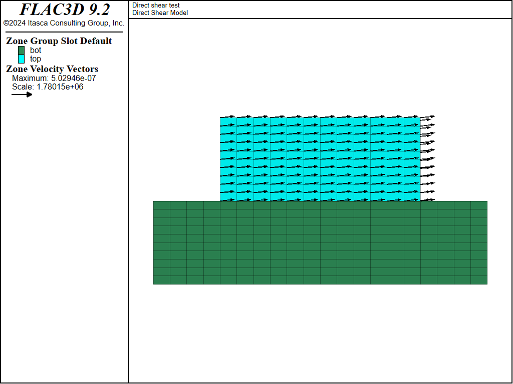
Figure 5: Direct shear test model.
First, a normal stress of 10 MPa that is representative of the confining stress acting on the joint is applied. A horizontal velocity is then applied to the top sub-grid to produce a shear displacement along the interface. For demonstration purposes, we only apply a small shear displacement of less than 2 mm to this model.
The average normal and shear stresses, and normal and shear displacements along the joint, are measured with a FISH function. With this information, we can determine the shear strength and dilation that are produced. To view this project, use the menu command . This is the the “DirectShearTest.prj” project.
DirectShearTest.dat
model new
model large-strain off
model title "Direct shear test"
fish automatic-create off
zone create brick size 12 1 10 point 0 4 0 5 point 1 16 0 5 ...
                               point 2 4 1 5 point 3 4 0 10 group 'top'
zone create brick size 20 1 10 point 1 20 0 0 point 2 0 1 0 ...
                               point 3 0 0 5 group 'bot' merge off
zone interface create by-face range group 'bot' position-z 5.0
zone interface node property stiffness-shear 4e4 stiffness-normal 4e4 ...
                             friction 30 dilation 6 ;tension 1e10 bslip=on
zone cmodel assign elastic
zone property bulk 45e3 shear 30e3
zone gridpoint fix velocity range position-z 0
zone gridpoint fix velocity-x range union position-x 0 position-x 20
zone face apply stress-normal -10 range position-z 10
model step 0
model solve
model save 'dsta.f3sav'
;
zone gridpoint fix velocity-x 5e-7 range group 'top'
program call 'fishFunctions'
[ini_jdisp]
history interval 10
fish history sstav
fish history nstav
fish history sjdisp
fish history njdisp
zone gridpoint initialize displacement (0,0,0)
model step 2500
model save 'dst.f3sav'
The average shear stress versus shear displacement along the joint is plotted in Figure 6, and the average normal displacement versus shear displacement is plotted in Figure 7. These plots indicate that joint slip occurs for the prescribed properties and conditions. The loading slope in Figure 6 is initially linear, and then becomes nonlinear as interface nodes begin to fail until a peak shear strength of approximately 5.8 MPa is reached. As indicated in Figure 7, the joint begins to dilate when the interface nodes begin to fail in shear.
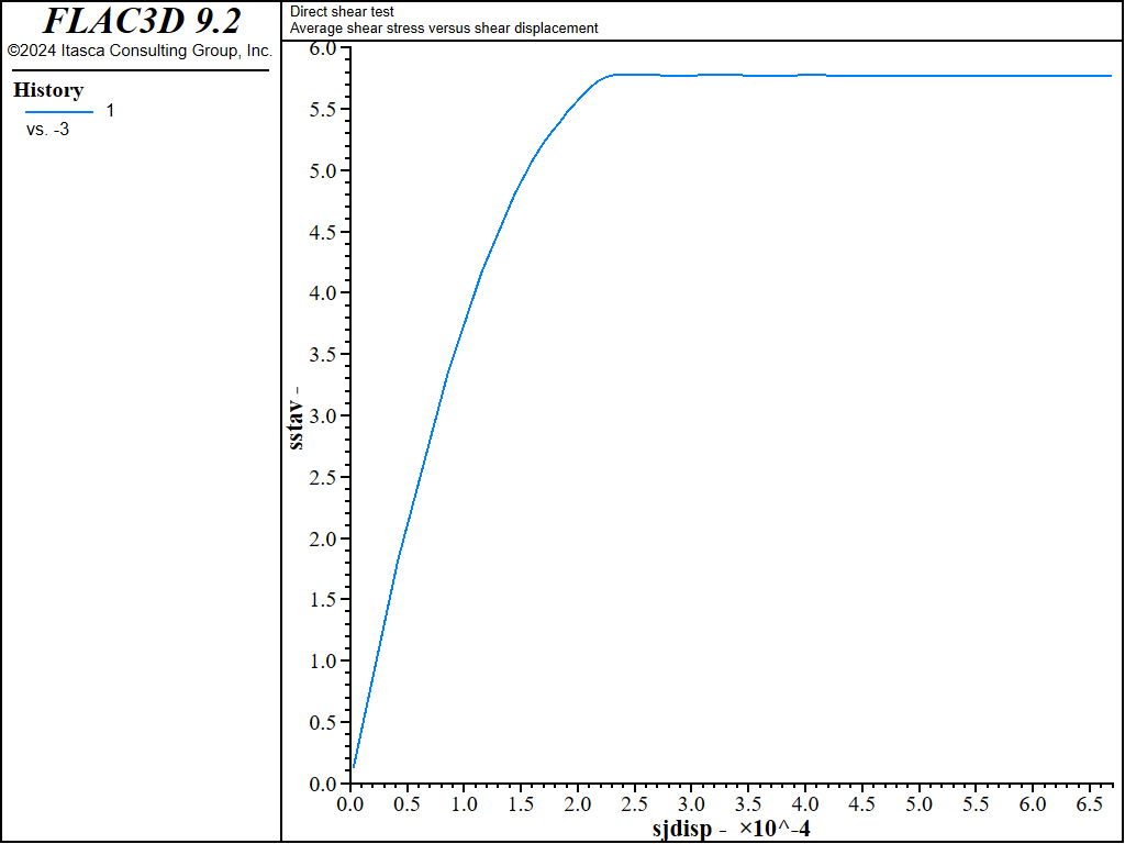
Figure 6: Average shear stress versus shear displacement.
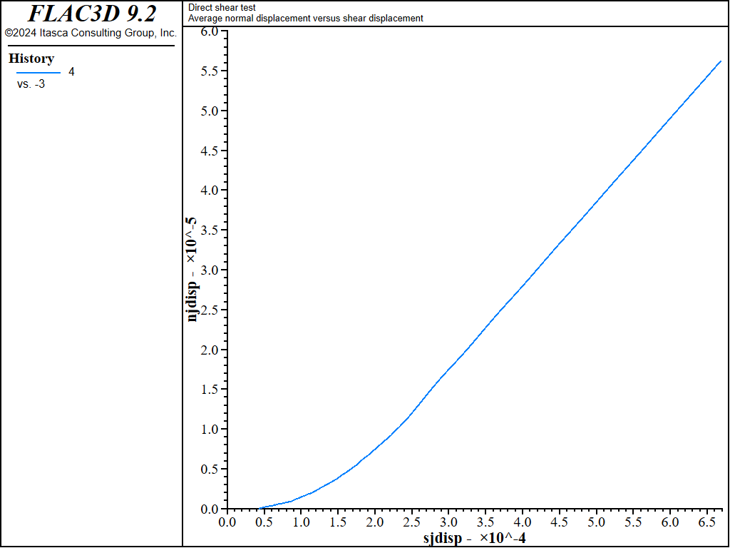
Figure 7: Average normal displacement versus shear displacement.
We can illustrate the influence of pore pressure on slip failure in a joint, by conducting a uniaxial compression test on the FLAC3D model of a specimen with a single joint that we created in “DippingJoint.dat”. The properties of the joint specimen are
normal stiffness (\(k_n\)) |
1 GPa/m |
shear stiffness (\(k_s\)) |
1 GPa/m |
cohesion (\(c_j\)) |
1 kPa |
friction angle (\(\phi_j\)) |
30° |
dilation angle (\(\psi_j\)) |
0° |
tensile strength (\(T_j\)) |
10 GPa |
The properties of the intact material are
Young’s modulus (\(E\)) |
170 MPa |
Poisson’s ratio (\(\nu\)) |
0.22 |
cohesion (\(c\)) |
2 kPa |
friction angle (\(\phi\)) |
40° |
dilation angle (\(\psi\)) |
0° |
tensile strength (\(T\)) |
2.4 kPa |
Slip will occur in a triaxial test, provided \((1- \tan\phi_j \tan\beta)\) 0 (Jaeger and Cook 1979), where \(\beta\) is the angle between the vertical direction and the joint plane. Assuming failure occurs due to slip along the joint, the peak stress, \(\sigma_1\), for the uniaxial compression test is related to the strength properties of the joint by the following expression (see Jaeger and Cook 1979):
where \(p\) is the constant pore pressure applied to the specimen (i.e., an undrained compression test, but with zero fluid modulus); \(\beta\) = 45° in this case. We perform two simulations to evaluate the influence of the pore pressure, \(p\), on the peak stress \(\sigma_1\). For the given material properties, and with \(p\) = 0, \(\sigma_1\) = -4.7 kPa. If we specify a pore pressure of 1.0 kPa, then \(\sigma_1\) = -2.0 kPa.
The data file to run a uniaxial test on the jointed specimen is contained in “UniaxialCompTest.dat”. The project file, “UniaxialCompTest.prj”, is located in the folder “datafiles\Interface\UniaxialCompTest.dat”
Two FISH functions (stress and strain) are used to calculate the stress-strain response during the test. The results are compared to the values calculated from Equation (5), which are stored as the FISH parameter analytical. Note that the tensile strength of the joint is set to a high value, but the property switch bonded-slip is set to on to allow slip along the joint.
UniaxialCompTest.dat
model new
model large-strain off
model title "Influence of pore pressure on slip failure in a joint"
fish automatic-create off
; Create Base
zone create brick size 3 3 3 ...
            point 0 (0,0,0) point 1 (3,0,0) point 2 (0,3,0) ...
            point 3 (0,0,1.5) point 4 (3,3,0) point 5 (0,3,1.5) ...
            point 6 (3,0,4.5) point 7 (3,3,4.5) group 'Base'
; Create Top - 1 unit high for initial spacing
zone create brick size 3 3 3 ...
point 0 (0,0,1.5) point 1 (3,0,4.5) point 2 (0,3,1.5) point 3 (0,0,6) ...
point 4 (3,3,4.5) point 5 (0,3,6) point 6 (3,0,6) point 7 (3,3,6) group 'Top'
; Create interface elements on the top surface of the base
zone interface create by-face separate range group 'Base' group 'Top'
; Assign Material model, continuum properties, and interface properties
zone cmodel assign mohr-coulomb
zone property bulk 1e8 shear 7e7 friction 40 cohesion 2e3 tension 2400
zone interface node property stiffness-normal 1e9 stiffness-shear 1e9 ...
                             friction 30 cohesion 1e3 tension 1e10 ...
                             bonded-slip on
; Fix upper and lower boundaries, and assign velocity
zone gridpoint fix velocity-z -5e-9 range position-z 6
zone gridpoint fix velocity-z  5e-9 range position-z 0
[global zpnt1 = gp.near(0,0,0)]
[global zpnt2 = gp.near(0,0,6)]
[global analytical = 4.732e3]
program call 'fishFunctions'
;
model history mechanical unbalanced-maximum
fish history stress
fish history analytical
fish history strain
model save 'state1'
;
model cycle 24000
model save 'slip_p0'
The stress-strain results for zero pore pressure are plotted in Figure 8, and for \(p\) = 1.0 kPa in Figure 9. The figures also show that the peak stresses calculated by FLAC3D compare well with the peak stresses calculated from Equation (5). The FLAC3D results can be further improved if a servo-control is used with the applied velocity to restrict the maximum unbalanced force as the joint begins to slip.
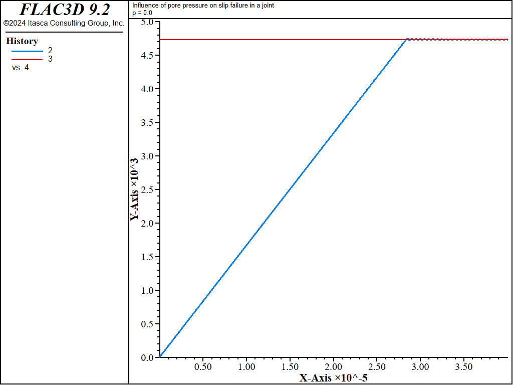
Figure 8: Stress-strain response of a jointed specimen, p = 0.0.
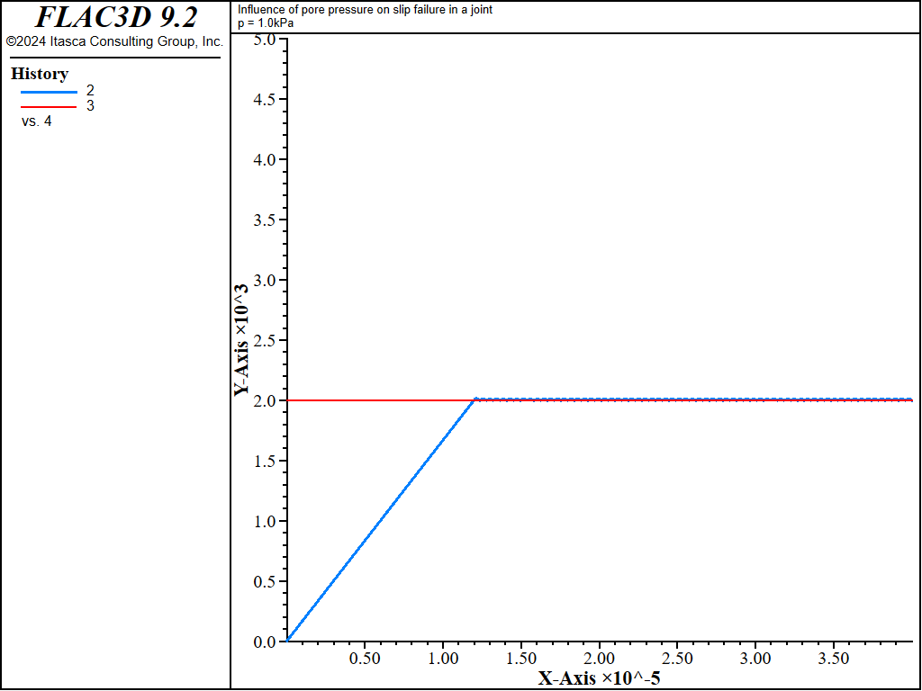
Figure 9: Stress-strain response of a jointed specimen, p = 1.0 kPa.
Endnotes
| Was this helpful? ... | Itasca Software © 2024, Itasca | Updated: Dec 05, 2024 |
