Rainfall on a Slope (FLAC2D)

Problem Statement

Note

This project reproduces Example 16 from FLAC 8.1. The project file for this example is available to be viewed/run in FLAC2D.[1] The project’s main data files are shown at the end of this example.

In this example, the stability of a generic slope is analyzed for two successive rainfall events of increasing intensity and decreasing duration. The slope geometry and location of the initial water table are shown in Figure 1. This corresponds to a constant rainfall rate of 84 mm/month. In the second event, nine inches (228 mm) of rain fall within four days. The purpose of this analysis is to determine the effect of each event on the stability of the slope.

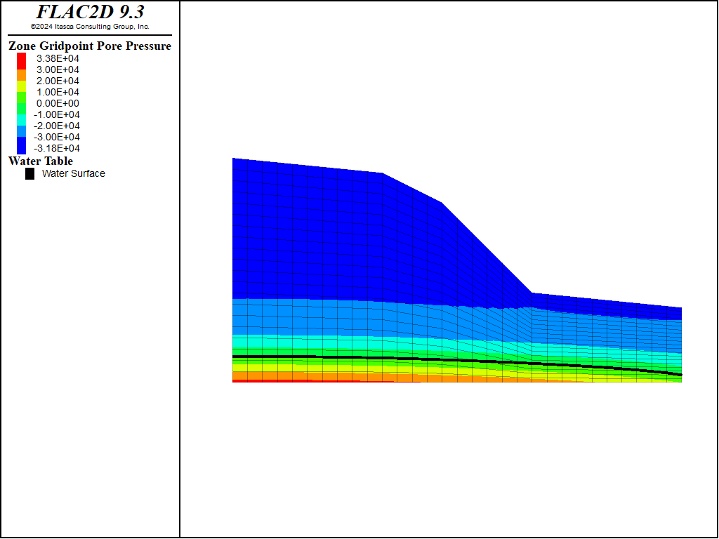
Figure 1: Pore pressure distribution for constant rainfall of 84 mm/month.

The presence of capillary pressure in unsaturated soils can have a big impact on the stability of a slope. Capillary forces hold fine particles together and can provide additional apparent cohesion to the soil. The apparent cohesion provided by the capillary forces usually decreases as the soil saturation increases. While a rainfall event of low intensity and long duration may, under certain conditions, be beneficial to the stability of the slope, a high-intensity, short-duration event may promote a buildup of saturation and induce slope failure. This example illustrates the dependency of the rate of infiltration from precipitation on the stability in a generic silty slope.

Modeling Procedure

Model Geometry

The model is 60 m wide, the highest elevation from the base is 30 m (left side of model), and the shortest is 10 m (right side of model). The flat part of the valley, included in the model, is 20 m wide.

The grid for this analysis can be created in the Sketch workspace by following these steps:

1. Create a new sketch.

2. Draw a polyline clicking on the following points: (0,0) (60,0) (60,10) (40,12) (28,24) (20,28) (0,30) (0,0).

3. To ensure a structured mesh, draw vertical lines as shown.

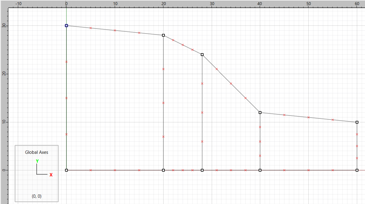
4. In the meshing menu, select Auto-size and set the value for model extent to 30.

5. Select all of the vertical lines and set the zone number to 20.

6. Mesh all polygons.

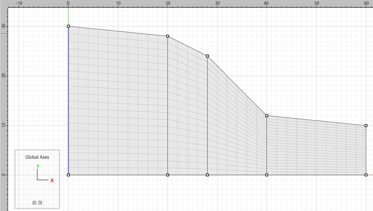
7. Create zones and save the project and the model state.

Properties

The slope is composed of silty soil, which is modeled as a Mohr-Coulomb material with zero cohesion and a 30º friction angle. The material and fluid properties assumed for this problem are listed in Table 1 and Table 2.

Table 1: Soil Properties

Property	Value
Dry Density (kg/m³)	2000
Drained bulk modulus (MPa)	200
Shear modulus (MPa)	100
Drained cohesion (Pa)	0
Drained friction angle (degrees)	30

Table 2: Fluid Properties

Property	Value
Fluid Density (kg/m³)	1000
Fluid modulus (MPa)	1
Porosity	0	.1
Hydraulic conductivity (m/s)	10	⁻⁵
van Genuchten parameter m	0	.336
van Genuchten parameter n	1	.506
van Genuchten parameter P_0 (MPa)	0	.015

The van Genuchten parameters are taken from the original FLAC 8.1 example that uses two-phase flow. For this example, an equation relating negative pore pressure (\(P_w\)) to saturation (\(S_e\)) is given:

\[-P_w = P_0 \left[S_e^{-1/a} - 1 \right]^{1-a}\]

where \(P_0\) is a reference pressure and \(a\) is a fitting parameter. This can be rearranged to give the equation for saturation versus pressure as shown here (Saturated/Unsaturated Flow, Using Simple-Fluid Mode) and reproduced below:

\[\hat{s} = \frac{1}{\left[ 1 + \left( \frac{\psi}{\psi_r} \right)^n \right]^m}\]

In this equation, \(m\) is equivalent to \(a\), \(n\) is equivalent to \(1 \over {1-a}\), \(\psi\) and \(\psi_r\) are equivalent to \(P_w\) and \(P_0\). The curve for these parameters is shown in Figure 4.

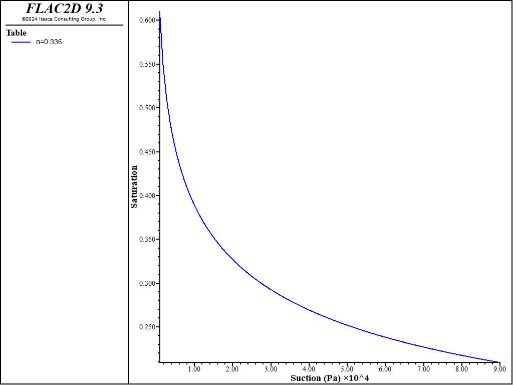
Figure 4: van Genuchten soil-suction curve for m = 0.336, n = 1.506 and \(P_0\) = 0.015 MPa.

In addition, the FLAC 8.1 example uses the following relationship between relative permeability (\(\kappa^w\)) and saturation (\(S_w\)):

\[\kappa^w = S_w^b \left[1-\left(1-S_w^{1/a} \right)^a \right]^2\]

In the example, a value of \(b\) = 0 is assumed. This permeability relationship is implemented in FLAC2D by creating a table of values that is input to the zone fluid permeability-saturation command. The resulting table is shown in Figure 5.

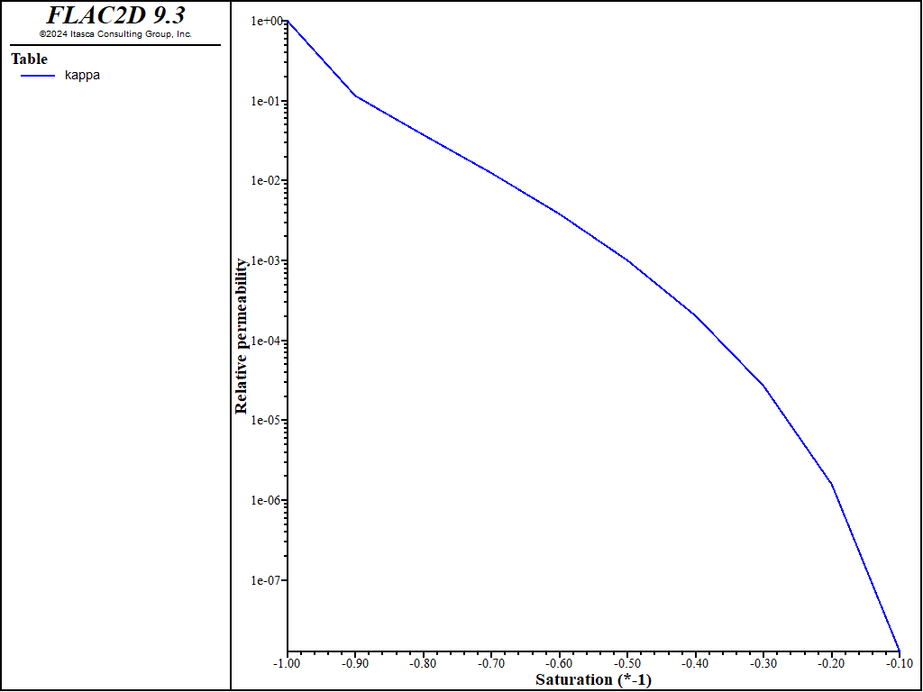
Figure 5: van Genuchten soil-suction curve for m = 0.336, n = 1.506 and \(P_0\) = 0.015 MPa.

First Rainfall Event: Low Intensity, Long Duration

It is assumed that rain falls at a constant rate of 84 mm/month (3.22e-8 m/s). Because rain falls vertically, and discharge is applied perpendicular to the faces, a simple FISH function is used to scale the applied discharge on the non-horizontal top surfaces. It is also assumed that the water table is at 1 m on the right side of the model (toe of the slope). The model is solved to steady state and the pore pressures are shown in Figure 1 above. Saturation contours are shown in Figure 6. It can be seen that the majority of the slope is not fully saturated and has negative pore pressure (suction). This means that the slope is mechanically stable, even though the steepest slope angle (45º) is higher than the friction angle (30º). The displacements are shown in Figure 7.

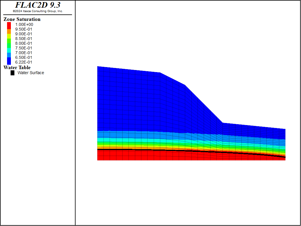
Figure 6: Saturation contours for constant, low intensity rainfall.

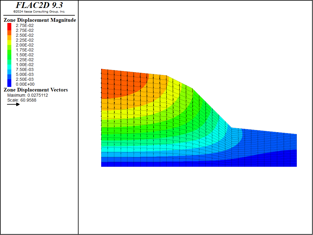
Figure 7: Displacements calculated for constant, low intensity rainfall.

Second Rainfall Event: High Intensity, Short Duration

The second rainfall event corresponds to an additional 228 mm (nine inches) of rainfall over a period of four days. A coupled numerical simulation is conducted to cover the time scale of this event. The slope is failing in this case. The velocity at the end of the simulation are shown in Figure 8. Contours of saturation are shown in Figure 9.

Saturation at the ground surface is seen to increase at the top half of the slope consistent with the higher magnitude of the current rainfall event. The increase of saturation is responsible for the subsequent reduction in apparent soil cohesion and ultimate failure of the slope.

Figure 8: Velocities after the short, high intensity rainfall.

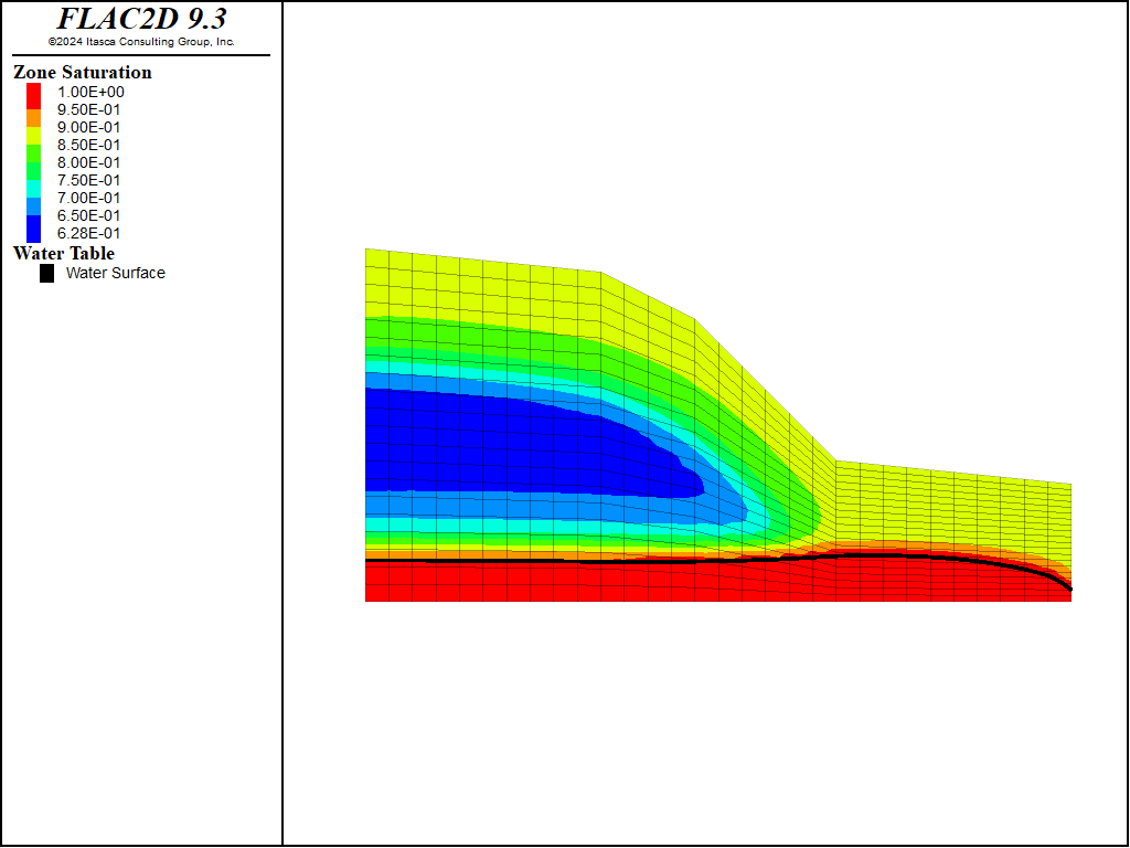
Figure 9: Saturation contours and flow vectors after the short, high intensity rainfall.

Discussion

Coupled numerical simulations of unsaturated seepage flow were performed to show the impact of intensity and duration of a rainfall event on the stability of a slope. Generic geometry and material properties were used for the slope. It was shown that a rainfall event of low intensity and long duration was not detrimental to slope stability, provided the suction due to the soil capillary forces was sufficient. On the other hand, a rainfall event of high intensity and short duration was responsible for slope failure. In this case, the behavior was explained by an increase in soil saturation, accompanied by a decrease in the intensity of capillary forces, causing an apparent decrease in soil cohesion.

Data Files

initial.dat

model new
program call 'sketch'
model save 'sketch'

model configure fluid-flow

; properties
zone cmodel assign mohr-coulomb
zone property density 2000 bulk 2e8 shear 1e8 friction 30

model gravity 9.81

zone fluid-density 1000
zone fluid property porosity 0.1 hydraulic-conductivity 1e-5
zone fluid property fluid-modulus 1e6
zone fluid unsaturated van-genuchten [1/(1-0.336)] 0.336 15000

; make a table for relative permeability - assume b = 0
fish define kappa(a)
  local tab = table.create('kappa')
  loop local i (1,10)
    local sat = i*0.1
    table(tab,sat) = sat*(1-(1-sat^(1/a))^a)^2
  end_loop
end
[kappa(0.336)]

zone fluid permeability-saturation table 'kappa'

; boundary conditions
zone face skin
zone face apply velocity-x 0 range group 'East' or 'West'
zone face apply velocity 0 0 range group 'Bottom'

; Discharge is applied normal to the face,
;   so we have to correct for face angle.

; input is zone pointer and side
; function will return a multiplier (0-1)
fish define dis_vert(zp,side)
    dis_vert = math.abs(zone.face.normal(zp,side)->y)
end

zone face apply discharge 3.22e-8 fish-local dis_vert range group 'Top'

; assume water table at 1 m on the right side
zone face apply head 1 range group 'East' position-y 0 1

zone fluid steady-state

model save 'initial-fluid'

; make sure suctions are included in effective stress calculations
zone fluid property effective-cutoff -1e20

model large-strain off
model solve-static elastic
model save 'initial'

heavy_rain.dat

model restore 'initial'

zone face apply discharge 6.6e-7 fish-local dis_vert range group 'Top'

zone history name 'pp middle' pore-pressure position 6,17
zone history name 'pp top' pore-pressure position 6,28
zone history name 'sat middle' saturation position 6,17
zone history name 'sat top' saturation position 6,28
model history fluid time-total

zone history name 'disp at crest' displacement position 28,24
zone history name 'vel at crest' displacement position 28,24

; fully coupled solution - solve fluid and mechanical simultaneously
; limit number of mechanical steps per fluid step, since model fails
model mechanical substep 10
model solve-fluid-coupled time [4*24*60*60] 

model save 'heavy_rain'

Endnote

[1]

This example is listed under the present document title in the i Examples dialog (use the menu command Help -> Examples… to access).