Examples • Example Applications

Swelling of a Fully Wetted Slope (FLAC2D)

Problem Statement

Note

This project reproduces Example 19 from FLAC 8.1. The project file for this example is available to be viewed/run in FLAC2D.[1] The project’s main data files are shown at the end of this example.

This example illustrates the estimation of volume change (swelling deformation) of a fill slope subjected to post-construction wetting. Swelling deformations are calculated using the swell constitutive model. The example is based upon an actual field case of a fill slope presented by Noorany et al. (1999).

The problem conditions correspond to a fully wetted fill slope. The slope is composed of three layers of fill material with different elastic, plastic, and wetting properties. The slope height is approximately 22 m, and the slope angle is roughly 24 degrees. The slope crest is at elevation 304.8 m. The top layer (soil 3) extends to elevation 293.0 m, the second layer (soil 4) extends to elevation 284.0 m, and the third layer (soil 5) extends approximately 3.0m to a slightly angled rock foundation. The slope face contains small 1.8-m wide benches at elevations 298.0 m and 284.0 m.

Relative horizontal movements between two points at two different sections on the fill slope crest were monitored when the slope was fully wetted. The monitoring points were approximately 26 m apart. The average swelling movement between points was found to be 103 mm.

Modeling Procedure

Model Geometry

The model zones are created in a sketch using the Slope Wizard tool. After opening the slope wizard, fill in the form as shown in Figure 1. Note that you don’t need to fill in the slope angles. Slope angle is automatically calculated in the dialog based on the other dimensions. Make sure you click in the slope angle boxes after filling in rise and run for each level and ensure that the numbers match those shown below. Also make sure to check the box at the bottom to Mirror layout and uncheck the box to Create internal edges.

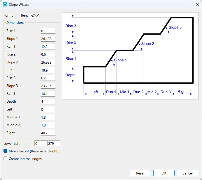
Figure 1: Slope Wizard entries used to create swelling slope geometry.

The resulting slope is shown in Figure 2.

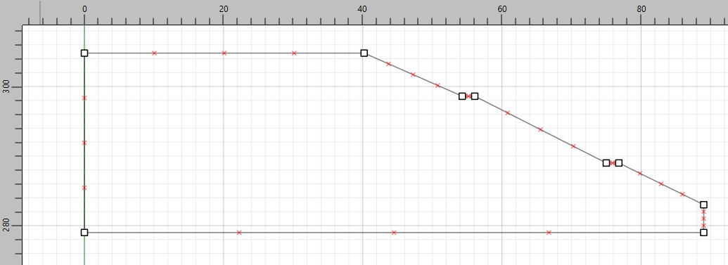
Figure 2: Slope created by Slope Wizard

Next, delete the bottom-right point (at x=89, y = 279). Draw a line to join the bottom-left point and bottom-right point.

Next we need to define the material layers. Draw horizontal lines at y=284 and y=293. The model should now appear as shown in Figure 3.

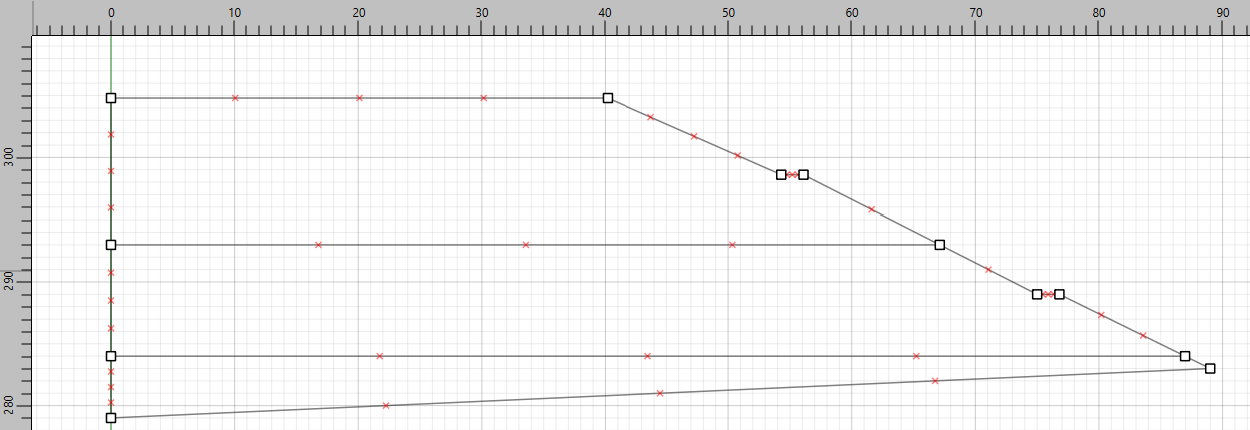
Figure 3: Slope after drawing the inclined bottom boundary and lines for material layers.

Next we mesh the model. Set the zone size to 1 and mesh all polygons. The model should appear as in Figure 4.

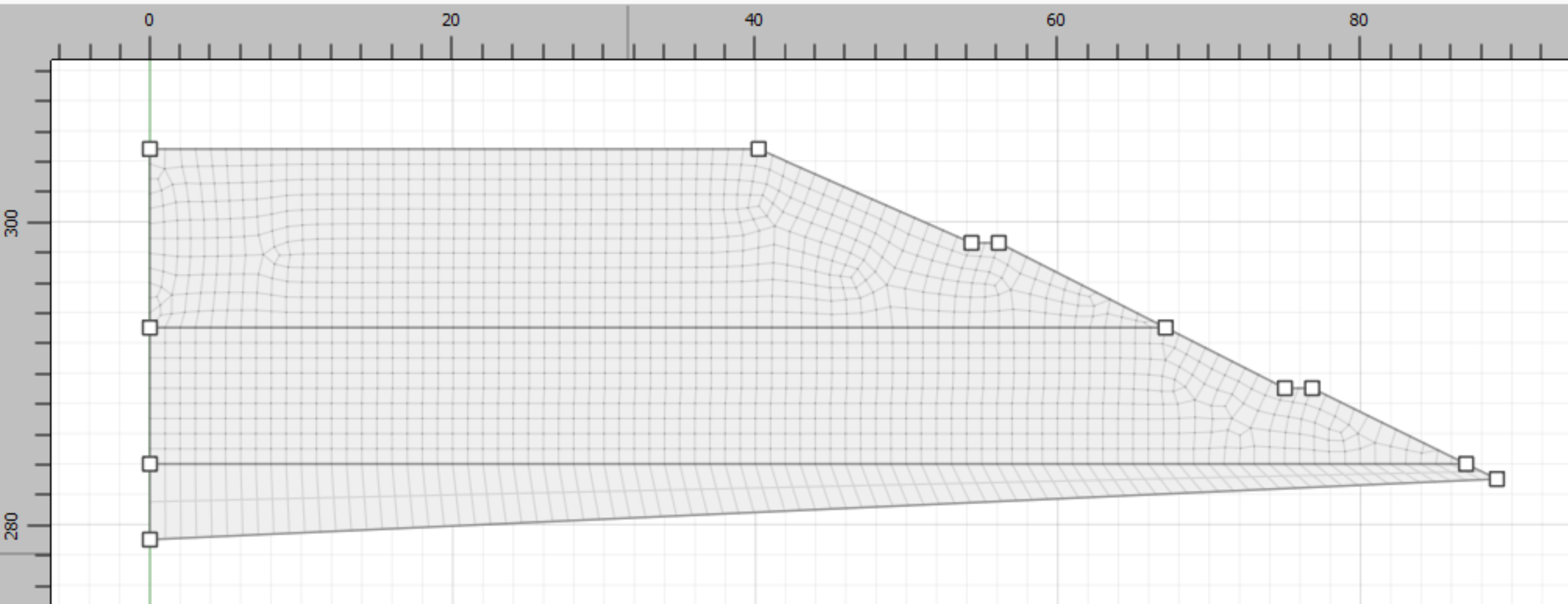
Figure 4: Slope after meshing.

Finally, we can define the material layers. Click on the top layer and set the group name to Soil3. Set the group name of the middle layer to Soil4 and the bottom to Soil5. Save the project and the model state. You may also wish to save the commands used to create the model. Do do this, click on the State Record tab at the bottom, right-click where you see the commands, and select .

Model Properties

The slope fill is modeled as Swell material. The constitutive model and properties can be set in the model pane, or by using commands. The assigned properties are shown in Table 1. Be careful to remain consistent with units. Stiffnesses are shown as kPa in Table 1 but Pa units are actually used in the example.

Table 1: Material Properties of Slope Soils

Soil	3	4	5
mass density (\(kg/m^3\))	1728.3	1575.4	1978.5
bulk modulus (kPa)	15400	32500	29300
shear modulus (kPa)	7120	15000	22000
friction angle (deg)	30	30	40
cohesion (kPa)	4.8	4.8	1.44
swelling type	logarithmic	logarithmic	linear
a1	1.533	0.694	0.0004
c1	-0.0187	-0.0211	0
a3	0.436	0.468	0.00047
c3	-0.0215	-0.023	0.001
m1	0.023	0.028	0.0
m3	0.036	0.036	0.0

Initially, the slope is considered to be un-wetted. The swell model requires an initial stress for each zone, so first the model must be solved with a mohr-coulomb material. We initially set the density, moduli and strength properties as shown in Table 1. The model is then solved.

The model is then changed to swell and all properties are assigned. For this example, principal swelling directions match the global coordinate system (angle = 0). Atmospheric pressure is set to 101.3 kPa, and swelling stresses are introduced over 20,000 steps.

Displacements and velocities for all gridpoints in the model are reset to zero, and the calculation is continued to introduce swelling.

Simulation Results

Figure 5 shows the vectors of the displacements induced by full wetting of the slope. Figure 6 shows the history plots of x-displacement and y-displacement at the crest edge. The maximum horizontal movement (to the right) obtained at the edge of the crest is ~131 mm. Swell (vertical displacement) at the same location is ~84 mm.

It is possible to compare results of the FLAC2D simulation with field data (see Noorany et al., 1999). The relative horizontal movement obtained from the FLAC2D analysis between two points on top of the slope (x=13.5 and the crest, x=39.6) is found to be 103 mm. This shows good agreement with field data. The calculated movement is compared to the measured value in Figure 7.

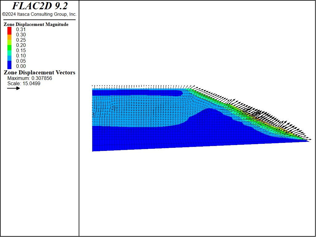
Figure 5: Displacements induced by wetting of the slope.

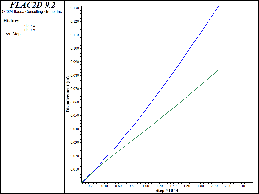
Figure 6: x- and y-displacement histories at crest edge.

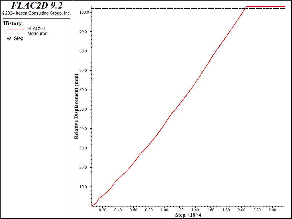
Figure 7: Comparison of calculated relative horizontal movement along the top of the slope compared to measured value.

Reference

Noorany, I., S. Frydman and C. Detournay. “Prediction of Soil Slope Deformation Due toWetting”, in FLAC and Numerical Modeling in Geomechanics, Proceedings of the First International FLAC Symposium (Minneapolis, September 1999), pp. 101-107, C. Detournay and R. Hart, Eds. Rotterdam: Balkema (1999).

Data Files

initial.dat

model new
program call 'sketch'

; assign Mohr-coulomb properties.  Swell properties are assigned later
; units are Pa
zone cmodel assign mohr-coulomb
zone property density 1728.3 bulk 15.4e6 shear 7.12e6 friction 30 ...
  cohesion 4800 range group 'Soil3'
zone property density 1575.4 bulk 32.5e6 shear 15.0e6 friction 30 ...
  cohesion 4800 range group 'Soil4'
zone property density 1978.5 bulk 29.3e6 shear 22.0e6 friction 40 ...
  cohesion 1440 range group 'Soil5'

; identify boundaries
zone face skin

; apply boundary conditions
zone face apply velocity-x 0 range group 'East' or 'West'
zone face apply velocity 0 0 range group 'Bottom'

; turn on gravity and solve
model gravity 9.81
model large-strain off
model solve elastic

model save 'initial'

swell.dat

model restore 'initial'

; reset displacements and velocities
zone gridpoint initialize displacement 0 0
zone gridpoint initialize velocity 0 0

; assign swell properties.  
zone cmodel assign swell

; MC properties
zone property density 1728.3 bulk 15.4e6 shear 7.12e6 friction 30 ...
  cohesion 4800 range group 'Soil3'
zone property density 1575.4 bulk 32.5e6 shear 15.0e6 friction 30 ...
  cohesion 4800 range group 'Soil4'
zone property density 1978.5 bulk 29.3e6 shear 22.0e6 friction 40 ...
  cohesion 1440 range group 'Soil5'

; swell properties

; these for all layers
zone property normal (0,1) pressure-reference 101.3e3 number-start 20000 

; these are layer-specific
zone property constant-a-1 1.533 constant-c-1 -0.0187 ...
              constant-a-3 0.436 constant-c-3 -0.0215 ...
              constant-m-1 0.023 constant-m-3 0.036 ...
              range group 'Soil3'
zone property constant-a-1 0.694 constant-c-1 -0.0211 ...
              constant-a-3 0.468 constant-c-3 -0.023 ...
              constant-m-1 0.028 constant-m-3 0.036 ...
              range group 'Soil4'
zone property constant-a-1 0.0004 constant-c-1 0 ...
              constant-a-3 0.00047 constant-c-3 0.001 ...
              flag-swell 2 ...
              range group 'Soil5'

; take histories at the crest
zone history name 'disp-x' displacement-x position 40.2,304.8
zone history name 'disp-y' displacement-y position 40.2,304.8

; get relative displacement between two locations
fish define xdisp_rel
  zone.field.name = 'displacement-x'
  ; displacements in mm
  local xdisp_right = zone.field.get(39.6,304.8)*1000
  local xdisp_left = zone.field.get(13.5,304.8)*1000
  xdisp_rel = xdisp_right - xdisp_left
  
  xdisp_meas = 102  ; field data
end

fish history name 'FLAC2D' xdisp_rel 
fish history name 'Measured' xdisp_meas 

model cycle 25000

model save 'swell'

Endnote

[1]

This example is listed under the present document title in the i Examples dialog use the menu command Help -> Examples… to access.