Hydrodynamic Pressure Acting on a Dam
Note
To view this project in FLAC3D, use the menu command . The main data files used are shown at the end of this example. The remaining data files can be found in the project.
A simple example is presented to illustrated the effect of hydrodynamic pressures on a concrete dam. The dynamic loading is applied in three different ways. First, the dam is subjected to a dynamic loading without taking into account the hydrodynamic pressure. Second, the hydrodynamic pressure is applied as a boundary condition by means of the Westergaard scaling of the grid point mass, as decribed in Hydrodynamic Pressures. Third, the hydrodynamic pressure is simulated by modeling the water directly as zones adjacent to the dam zones.
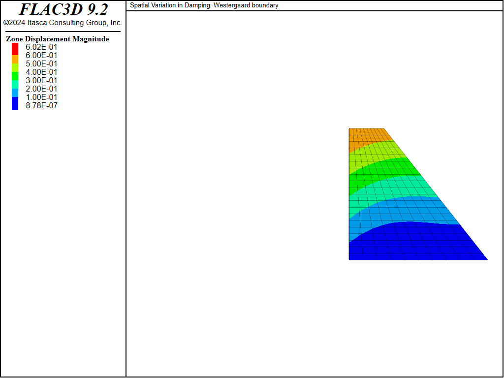
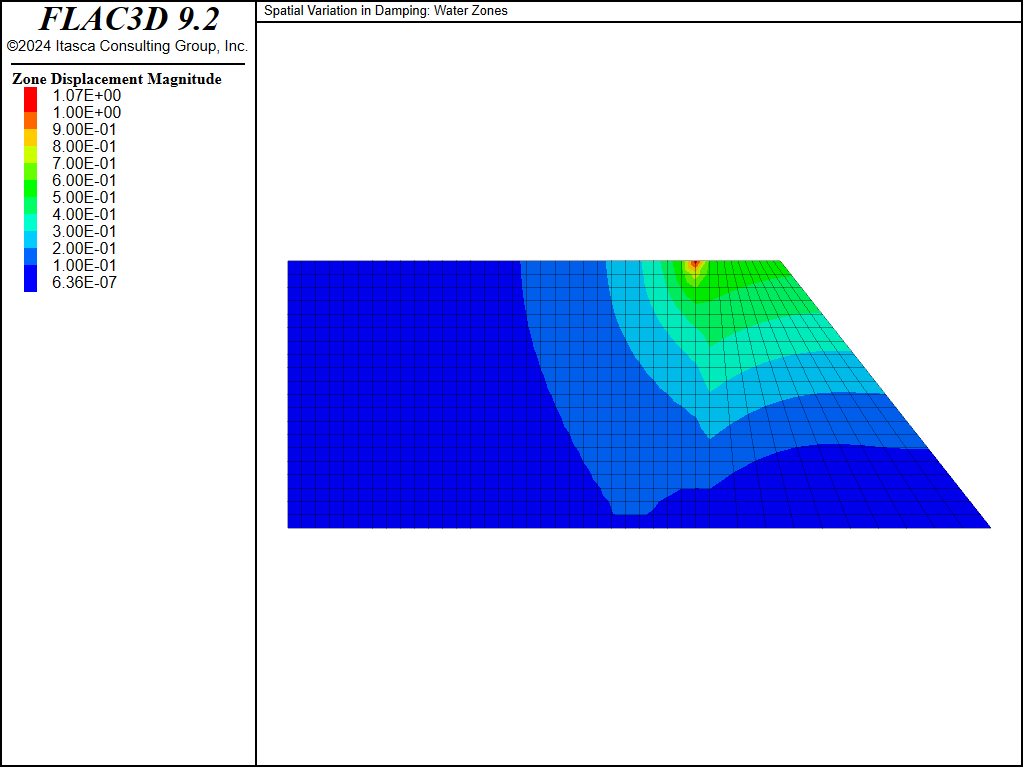
Figure 1 shows the geometry of the model for the first two loading cases, and Figure 2 shows the model for the third case.

Figure 1: Dam model with hydrodynamic pressure boundary on upstream face.

Figure 2: Dam model with water zones on upstream face.
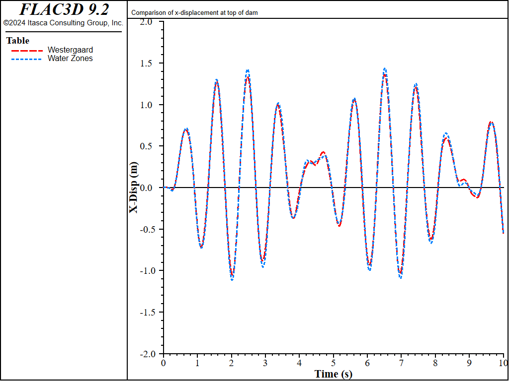
The dynamic loading is a velocity sine wave applied to the base of the model. The models are first brought to a static equilibrium state with the reservoir loading applied along the upstream vertical face of the dam. The dynamic loading is then applied for a period of 10 seconds. The horizontal displacement at the top of the dam at the upstream face is monitored for all three cases. The results are plotted for comparison in Figure 3.

Figure 3: Comparison of \(x\)-displacement at top of dam.
These results illustrate the effect on displacement of the hydrodynamic pressures. The case using the Westergaard adjustment is in good agreement with the case modeling the water explicitly.
Data Files
HydroDynamicPressureStress.dat
model new
model large-strain off
model configure dynamic
model title "Spatial Variation in Damping: Stress only"
; Create zones
zone create brick size 10 1 20 point 1 (20,0,0) point 2 (0,1,0) ...
    point 3 (0,0,19)   point 6 (5,0,19) point 7 (5,1,19) group "Dam"
; Assign constitutive model and properties
zone cmodel assign elastic
zone property density 2000 bulk 1e8 shear 3e7
; Boundary conditions
zone gridpoint fix velocity range position-z 0
zone gridpoint fix velocity-y
zone face apply stress-normal -190000 gradient (0,0,10000) range position-x 0.0
; Initial conditions
model gravity 10
zone initialize-stresses
; Solve to initial equilibrium
model dynamic off
model solve convergence 1
; Reset velocities and displacements
zone gridpoint initialize velocity (0,0,0)
zone gridpoint initialize displacement (0,0,0)
; Update boundary conditions
fish define sine_wave
    sine_wave = math.sin(2.0*math.pi*zone.dynamic.time.total)
end
zone gridpoint free velocity-x range position-z 0
zone face apply velocity-x 1.0 fish sine_wave range position-z 0
; Take some histories
model history name='time' dynamic time-total
zone  history name='xdisp' displacement-x position (0,0,19)
; Solve to time 10
model dynamic on
model solve time-total 10
model save 'Stress'
HydroDynamicPressureWestergaard.dat
model new
model large-strain off
model configure dynamic
model title "Spatial Variation in Damping: Westergaard boundary"
; Create zones
zone create brick size 10 1 20 point 1 (20,0,0) point 2 (0,1,0) ...
                               point 3 (0,0,19) point 6 (5,0,19) ...
                               point 7 (5,1,19) group "Dam"
; Assign constitutive model and properties
zone cmodel assign elastic
zone property density 2000 bulk 1e8 shear 3e7
; Boundary conditions
zone gridpoint fix velocity range position-z 0
zone gridpoint fix velocity-y
zone face apply stress-normal -190000 gradient (0,0,10000) range position-x 0.0
; Initial conditions
model gravity 10
zone initialize-stresses
; Solve to initial equilibrium
model dynamic off
model solve convergence 1
; Reset velocities and displacements
zone gridpoint initialize velocity (0,0,0)
zone gridpoint initialize displacement (0,0,0)
; Update boundary conditions
fish define sine_wave
    sine_wave = math.sin(2.0*math.pi*zone.dynamic.time.total)
end
zone gridpoint free velocity-x range position-z 0
zone face apply velocity-x 1.0 fish sine_wave range position-z 0
zone face westergaard direction (-1,0,0) height 19 base 0 ...
          density-water 1000 range position-x 0
; Take some histories
model history name='time' dynamic time-total
zone  history name='xdisp' displacement-x position (0,0,19)
; Solve to time 10
model dynamic on
model solve time-total 10
model save 'Westergaard'
HydroDynamicPressureWater.dat
model new
model large-strain off
model configure dynamic
model title "Spatial Variation in Damping: Water Zones"
; Create zones
zone create brick size 10 1 20 point 1 (20,0,0) point 2 (0,1,0) ...
                               point 3 (0,0,19) point 6 (5,0,19) ...
                               point 7 (5,1,19) group "Dam"
zone create brick size 30 1 20 point 0 (-30,0,0) point 1 (0,0,0) ...
                               point 2 (-30,1,0) point 3 (-30,0,19) ...
                               group "Water"
; Assign constitutive model and properties
zone cmodel assign elastic
zone property density 2000 bulk 1e8 shear 3e7 range group "Dam"
zone property density 1000 bulk 2e9 shear 0 range group "Water"
; Boundary conditions
zone gridpoint fix velocity range position-z 0
zone gridpoint fix velocity-y
zone gridpoint fix velocity-x range position-x -30
;zone face apply stress-normal -190000 gradient (0,0,10000)
; Initial conditions
model gravity 10
zone initialize-stresses
; Solve to initial equilibrium
model dynamic off
model solve convergence 1
; Reset velocities and displacements
zone gridpoint initialize velocity (0,0,0)
zone gridpoint initialize displacement (0,0,0)
; Update boundary conditions
fish define sine_wave
    sine_wave = math.sin(2.0*math.pi*zone.dynamic.time.total)
end
zone gridpoint free velocity-x range position-z 0
zone face apply velocity-x 1.0 fish sine_wave range position-z 0
; Take some histories
model history name='time' dynamic time-total
zone  history name='xdisp' displacement-x position (0,0,19)
; Solve to time 10
model dynamic on
model solve time-total 10
model save 'Water'
| Was this helpful? ... | Itasca Software © 2024, Itasca | Updated: Dec 05, 2024 |
