FLAC3D Theory and Background • Fluid-Mechanical Interaction

Unsteady Groundwater Flow in a Confined Layer

Note

To view this project in FLAC3D, use the menu command Help ► Examples…. The project’s main data files are shown at the end of this example.

A long embankment of width \(L\) = 100 m rests on a shallow saturated layer of soil. The width (\(L\)) of the embankment is large in comparison to the layer thickness, and its permeability is negligible when compared to the permeability, \(k\) = 10^-12 m²/(Pa sec), of the soil. The Biot modulus for the soil is measured to be \(M\) = 10 GPa. Initial steady-state conditions are reached in the homogeneous layer. The purpose is to study the pore-pressure change in the layer as the water level is raised instantaneously upstream by an amount \(H_0\) = 2 m. This corresponds to a pore-pressure rise of \(p_1 = H_0 {\rho}_w g\) (with the water density \({\rho}_w\) = 1000 kg/m³ and acceleration of gravity \(g\) = 10 m/s²) at the upstream side of the embankment. Figure 1 shows the geometry of the problem:

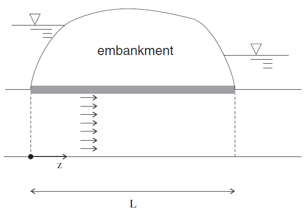
Figure 1: Confined flow in a soil layer.

The flow in the layer may be assumed to be one-dimensional. The model has width \(L\). The excess pore pressure, \(p\), initially zero, is raised suddenly to the value \(p_1\) at one end of the model. The corresponding analytical solution has the form

\[\hat{p}(\hat{z},t)\ =\ 1 - \hat{z} - {2 \over {\pi}} \sum_{n=1}^\infty e^{- n^2\pi^2 \hat{t}}\left({\sin {n \pi \hat{z}} \over n}\right)\]

where the \(z\)-axis is running along the embankment width and has its origin at the upstream side, \(\hat{p} = {p\over p_1}\), \(\hat{z} = {z \over {L}}\), \(\hat{t} = c t/L^2\), and \(c = M k\).

In the FLAC3D model, the layer is defined as a column of 25 zones. The excess pore pressure is fixed at the value of 2 × 10⁴ Pa at the face located at \(z\) = 0, and at zero at the face located at \(z\) = 100 m. The model grid is shown in Figure 2.

The analytical solution is programmed as a FISH function for direct comparison to the numerical results at selected fluid-flow times corresponding to \(\hat{t}\) = 0.05, 0.1, 0.2 and 1.0. The analytical and numerical pore-pressure results for these times are stored in tables.

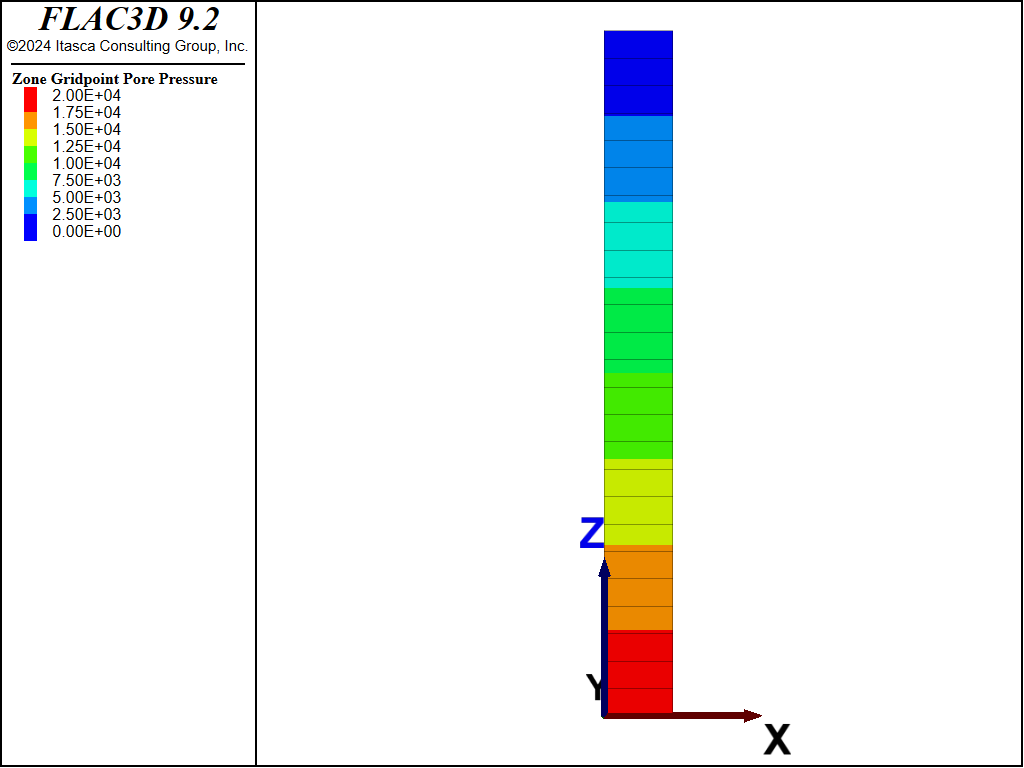
Figure 2: FLAC3D grid for fluid flow in a confined soil layer.

UnsteadyGroundwaterFlowConfinedLayer.dat contains the FLAC3D data file for this problem, using the implicit servo to automatically switch from explicit to implicit and increase the implicit timestep. UnsteadyGroundwaterFlowConfinedLayer-Steady.dat contains the data file using the zone fluid steady-state command to immediately find the steady state solution.

The comparison of analytical and numerical excess pore pressures at four fluid-flow times for the transient solution is shown in Figure 3. Normalized excess pore pressure (\(p/p_1\)) is plotted versus normalized distance (\(z/L\)) in the figure, where Tables 2, 4, and 6 contain the analytical solution for excess pore pressures, and Tables 1, 3, and 5 contain the FLAC3D solutions. The four flow times are 5 × 10⁴, 10⁵, 2 × 10⁵, and 10⁶ seconds. Steady-state conditions are reached by the last time considered. The difference between analytical and numerical pore pressures at steady state is less than 0.2%.

break

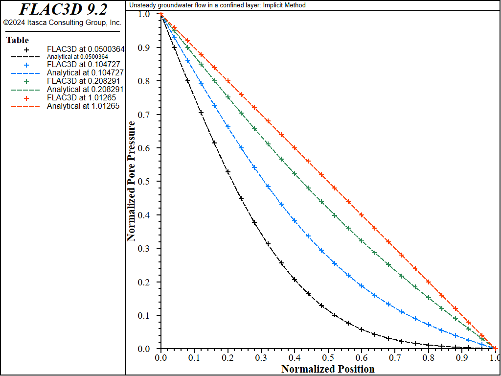
Figure 3: Comparison of excess pore pressures (analytical values = lines; numerical values = crosses).

Data File

UnsteadyGroundwaterFlowConfinedLayer.dat

model new
model title 'Unsteady groundwater flow in a confined layer: Implicit Method'
zone create brick size 1 1 25 point 1 (10 0 0) point 2 (0 10 0) ...
                              point 3 (0 0 100)
zone face skin                              
; --- fluid flow model ---
model configure fluid-flow
zone fluid property mobility-coefficient 1e-12 biot-modulus 1e10
zone face apply pore-pressure 2e4 range group 'Bottom'
zone face apply pore-pressure 0   range group 'Top'
; --- settings ---
zone results pore-pressure on
; Switch to implicit servo and increase dt automatically.
zone fluid implicit servo on 
model solve-fluid time 5e4
model results export 'confinedlayer-005'

model solve-fluid time 5e4
model results export 'confinedlayer-010'

model solve-fluid time 10e4
model results export 'confinedlayer-020'

model solve-fluid time 80e4
model results export 'confinedlayer-100'

model save 'confinedlayer'

SteadyState.dat

model new
model title 'Unsteady groundwater flow in a confined layer: Implicit Method'
zone create brick size 1 1 25 point 1 (10 0 0) point 2 (0 10 0) ...
                              point 3 (0 0 100)
zone face skin                              
; --- fluid flow model ---
model configure fluid-flow
zone fluid property mobility-coefficient 1e-12
zone face apply pore-pressure 2e4 range group 'Bottom'
zone face apply pore-pressure 0   range group 'Top'
; --- settings ---
zone fluid steady-state
;
model save 'confinedlayer-steadystate'