Examples • Verification Problems
Drained and Undrained Triaxial Compression Test on a Cam-Clay Sample (FLAC3D)
Problem Statement
Note
The project file for this example is available to be viewed/run in FLAC3D.[1] The main data files used are shown at the end of this example. The remaining data files can be found in the project.
Conventional drained and undrained triaxial compression tests on Cam-clay soil samples are modeled using FLAC3D. The stresses and specific volume at the critical state are compared with analytical predictions. The responses of both a lightly (LOC) and a heavily (HOC) over-consolidated specimen are considered. This set of problems tests the prediction accuracy of the modified Cam-clay model in FLAC3D.
The model of the sample is a cube with unit dimensions. The sample is made of a Cam-clay material with several properties:
shear modulus (\(G\)) |
250 \(p'_1\) |
soil constant (\(M\)) |
1.02 |
slope of normal consolidation line (\(\lambda\)) |
0.2 |
slope of elastic swelling line (\(\kappa\)) |
0.05 |
reference pressure (\(p'_1\)) |
1 kPa |
pre-consolidation pressure (\(p'_{c0}\)) |
8 \(p'_1\) and 40 \(p'_1\) |
specific volume at reference pressure on normal consolidation line (\(v_{\lambda}\)) |
3.32 |
Initially, the sample is in a state of isotropic compression corresponding to \(p_0 = 5 p'_1\) and zero excess pore pressure (\(p'_0 = p_0\)). The pre-consolidation pressure \(p'_{c0}\) has magnitude 8 × \(p'_1\) in the lightly over-consolidated case, and 40 × \(p'_1\) in the heavily over-consolidated case. These cases correspond to an over-consolidation ratio \(R = p'_{c0} / p'_0\) of 1.6 and 8, respectively. The shear modulus is assumed to remain constant during the test carried out with constant confining pressure \(p_0\) and simulated strain-controlled platens. Drained and undrained tests are considered. Refer to Wood (1990) for a detailed discussion on the Cam-clay plasticity theory.
Closed-Form Solutions
The mean pressure \(p\) and deviator stress \(q\) in a conventional triaxial test can be expressed as
where \(\sigma_1\) is the axial stress and \(-\sigma_2\) is the cell pressure.
Since the cell pressure is kept constant during the test, the total stress path in the \((p,q)\) plane is constrained by the relation
With initial conditions of the form \(p = p'_0\), \(q\) = 0, obtained upon integration is
In a drained test, no excess pore pressure is generated, the effective and the total stress paths coincide, and we may write
This stress path is represented in the figure below. The dashed line in the figure is the critical state line.
In an undrained test, when the fluid bulk modulus is much larger than that of the soil (incompressible fluid), the specific volume \(v\) remains constant, equal to the initial value \(v_0\), and it may be shown that the effective stress path is also well-defined.
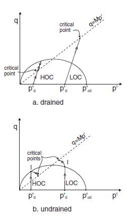
Figure 1: Effective stress paths.
Consider the case of an over-consolidated sample. Referring to (b) in the above figure, as long as the stress state lies inside the first yield surface, the path corresponds to the straight line,
When plastic deformation takes place, the shape of the effective stress path is given by (Wood, 1990, p. 127)
where \(\Lambda = (\lambda - \kappa) / \lambda\), \(\eta = q/p'\), and \(p'_i\) and \(\eta_i\) define the effective stress state at impending yield, indicated as point \(I\) in (b) in the figure above.
Note that, under undrained conditions, the yield path is defined by an equation of the form shown in equation (2) for any boundary condition (i.e., not only under triaxial compression conditions).
Intersection of the yield curve through \(p'_{c0}\) with the straight path \(p' = p'_0\) gives (using that \(R = p'_{c0}/p'_0\))
After substitution of those expressions in equation (2), we obtain
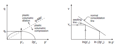
Figure 2: Critical state.
As the test proceeds, the path converges toward the critical state represented by the point \((p'_{cr},q_{cr})\) at the intersection with the critical state line \(q = M p'\) in the \((p',q)\) plane (see both figures above). The normal to the yield surface at the critical point is parallel to the \(q\)-axis. Because the plastic flow rule is associated, no more plastic volumetric strain can take place. Hence, no softening or hardening of the yield surface can occur; the ultimate yield surface corresponds to a \(p'_c\) value of \(2 p'_{cr}\), which is larger than \(p'_{c0}\) for a LOC sample, and smaller than \(p'_{c0}\) for a HOC sample. Unlimited plastic shear strains can develop at constant stresses, and also constant critical specific volume \(v_{cr}\).
In the drained case, the critical state is defined as
where the value \(v_{cr}\) corresponds to the specific volume at \(p = p_{cr}\) on the elastic swelling line through \(p_c = 2 p_{cr}\). In this case, the critical state of a specific material depends only on the initial mean pressure and is not affected by the pre-consolidation pressure.
In the undrained case, the intersection of the stress path represented by equation (3) with the critical state line \(\eta = M\) yields (assuming that \(v\) remains constant)
where \(v_0\) is the initial specific volume.
The excess pore pressure \(u\) is given by
Using equation (1) for the total pressure, we obtain
And, at the critical state,
FLAC3D Models
The numerical tests are carried out using one single zone with unit dimensions. The grid is fixed in the \(z\)-direction, and a velocity boundary condition applied at the top of the model. An initial isotropic compressive stress of 5 × \(p'_1\) is prescribed, and a constant lateral confining pressure \(p_0 = 5 \times p'_1\) is imposed in the \(x\)- and \(y\)-directions. To run the undrained examples, the fluid configuration is selected and flow calculations are turned off.
The initial specific volume is calculated internally (default value) to correspond with the value on the swelling line at the pre-consolidation pressure \(p'_{c0}\) and mean pressure \(p_0\):
The bulk modulus, \(K\), is initialized by the code to the value
The maximum value of the tangent bulk modulus is set to 800 × \(p'_1\).
A total of 10,000 cycles with a velocity magnitude of 0.5 × 10⁻⁴ m/sec was used in the drained examples. For the undrained tests, a compressive velocity of magnitude 0.5 × 10⁻⁶ m/sec is applied for the first 20 out of every 40 steps at the top of the model, and to zero for the remaining 20 steps. A total of 40,000 cycles are used. Biot modulus is set to 2 × 10⁴ × \(p'_1 /n\) (a large value compared to the initial value of the bulk modulus, which is of the order 102 × \(p'_1\)). (The porosity n is derived from the specific volume using \(n = (v-1/v\)).) The mean pressure, deviatoric stress, specific volume, and, in the undrained case, pore pressure are monitored as they converge to the critical state.
FLAC3D Results and Discussion
Numerical values for \(p'_1\), \(q\), \(v\), and \(u\) at the end of the simulation are compared with the analytical predictions. The results, presented in Table 2 and Table 3, indicate relative errors of less than 2%.
R = 1.6 |
R = 8 |
Analytical |
|
|---|---|---|---|
\(p\) |
7.573 |
7.583 |
7.576 |
\(q\) |
7.718 |
7.747 |
7.727 |
\(v\) |
2.811 |
2.811 |
2.811 |
R = 1.6 |
R = 8 |
|||
|---|---|---|---|---|
Numerical |
Analytical |
Numerical |
Analytical |
|
\(p'_1\) |
4.234 |
4.229 |
14.05 |
14.14 |
\(q\) |
4.312 |
4.314 |
14.42 |
14.43 |
\(v\) |
2.927 |
2.928 |
2.687 |
2.686 |
\(u\) |
2.203 |
2.209 |
-4.241 |
-4.334 |
The diagrams \((p',q)\) and \((\ln p',v)\) for the different tests are presented in Figure 3 to Figure 10. The responses of the lightly and heavily over-consolidated samples on their way to the critical state are in agreement with those predicted by the theory.
As the drained test progresses, the lightly over-consolidated sample shows a steady increase in deviator stress \(q\), and a steady decrease in specific volume. The heavily over-consolidated sample shows a rise in deviatoric stress to a peak followed by a drop, and an initial decrease in volume followed by volumetric expansion (see Figure 11 through Figure 14). The principal feature of the undrained tests is the contrast between the steady increase of pore pressure in the lightly over-consolidated sample, and the initial increase followed by a steady decrease of pore pressure in the heavily over-consolidated soil (see Figure 15 and Figure 16).
The data files “drained.dat” and “undrained.dat” were used to carry out the drained and undrained numerical tests. The file “TriaxialCompressionTest.dat” was used to set the property mpc to the values 8 and 40 to treat the lightly and heavily over-consolidated cases, respectively. FISH functions are used to apply the velocity boundary conditions and evaluate the relative error made at the end of the simulation.
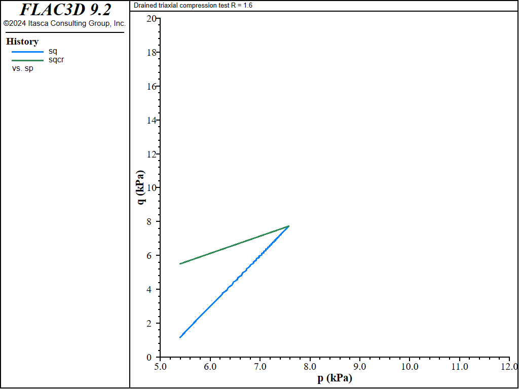
Figure 3: Stress path for R = 1.6—drained test.
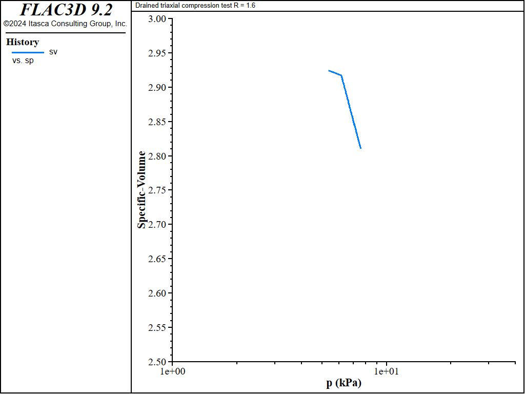
Figure 4: Diagram (\(\ln p, v\)) for R = 1.6—drained test.
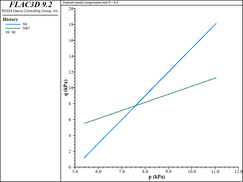
Figure 5: Stress path for R = 8—drained test.
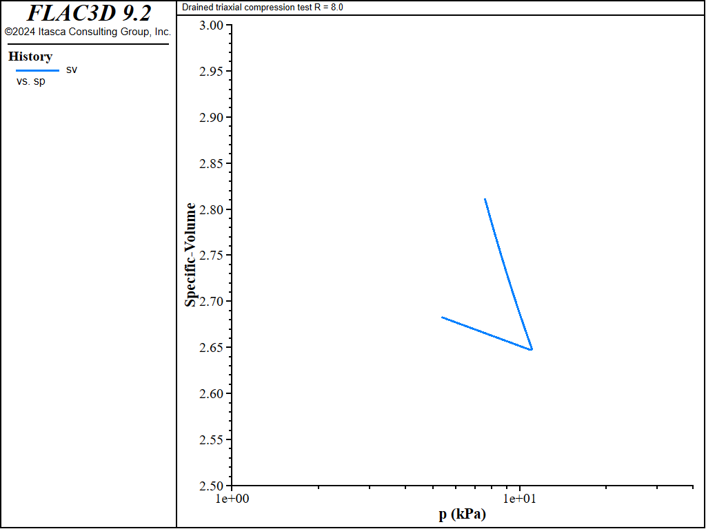
Figure 6: Diagram for (\(\ln p, v\)) for R = 8—drained test.
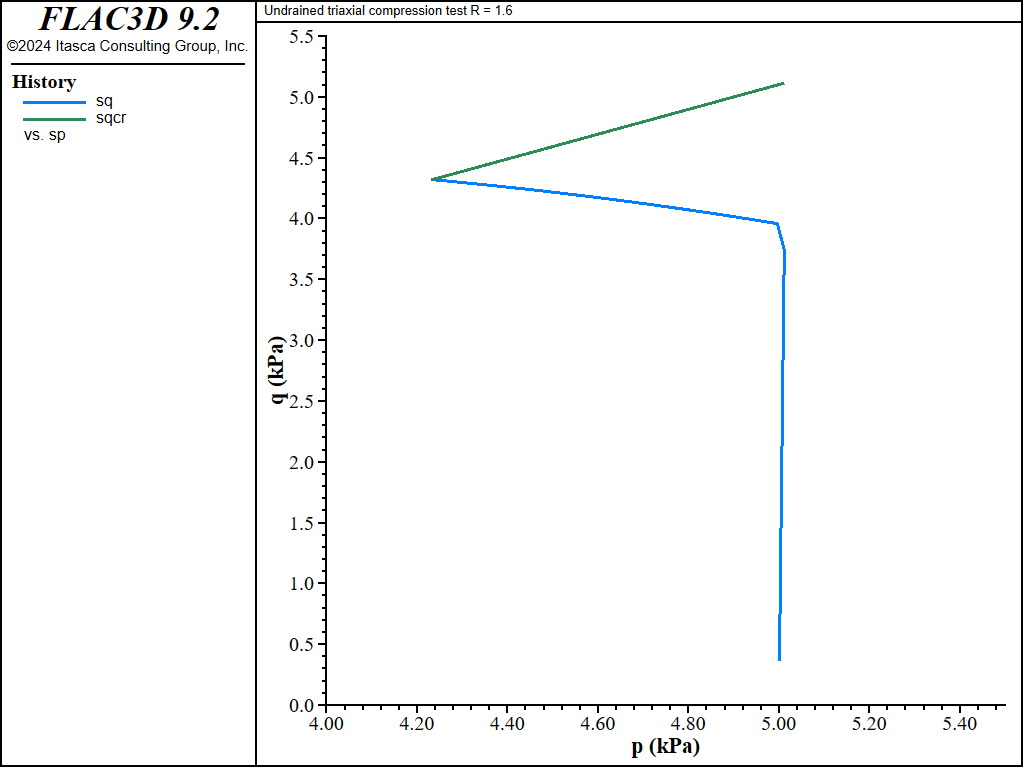
Figure 7: Stress path for R = 1.6—undrained test.
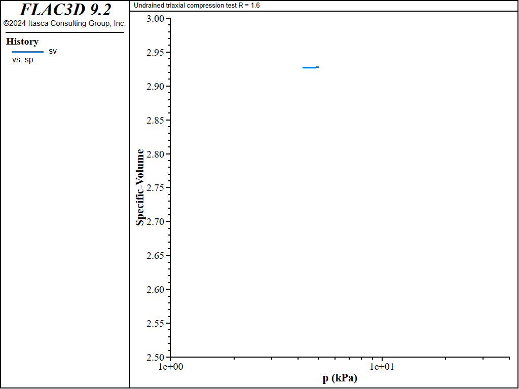
Figure 8: Diagram for (\(\ln p, v\)) for R = 1.6—undrained test.
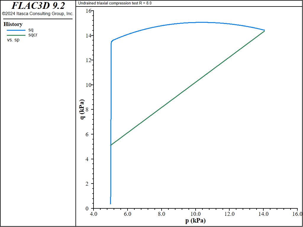
Figure 9: Stress path for R = 8—undrained test.
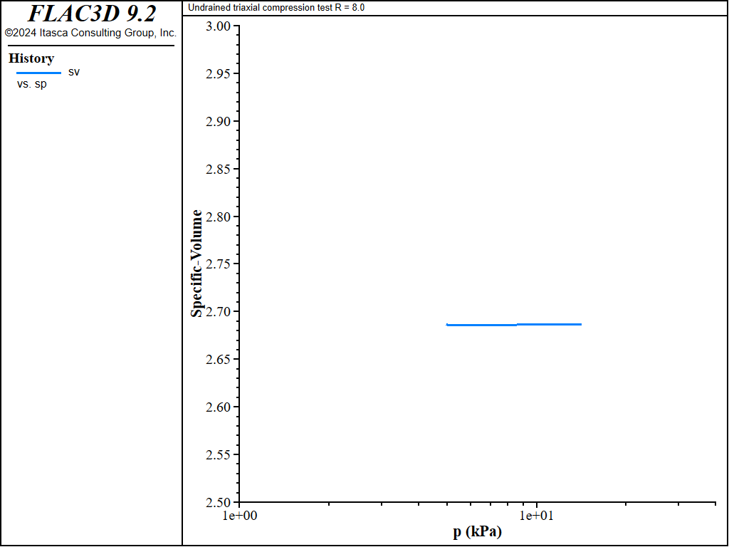
Figure 10: Diagram for (\(\ln p, v\)) for R = 8—undrained test.
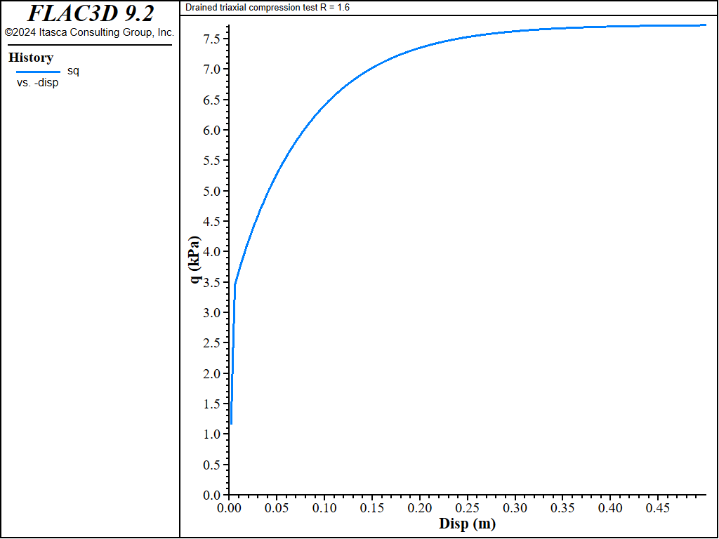
Figure 11: Evolution of deviator stress with axial strain for R = 1.6—drained test.
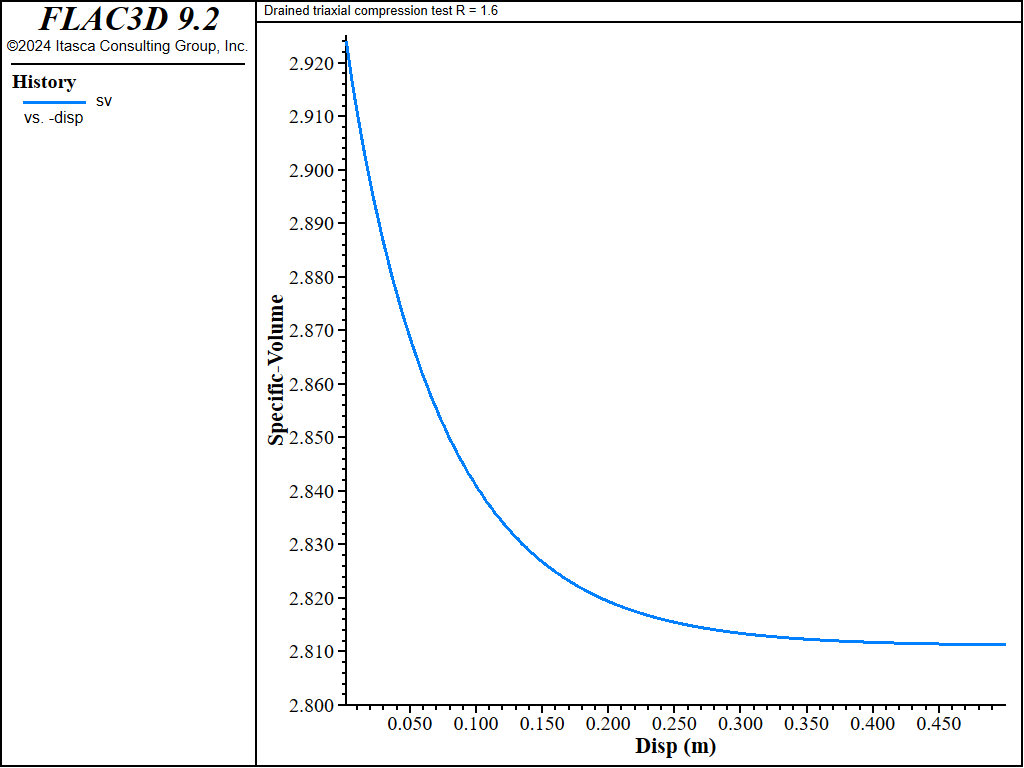
Figure 12: Evolution of specific volume with axial strain for R = 1.6—drained test.
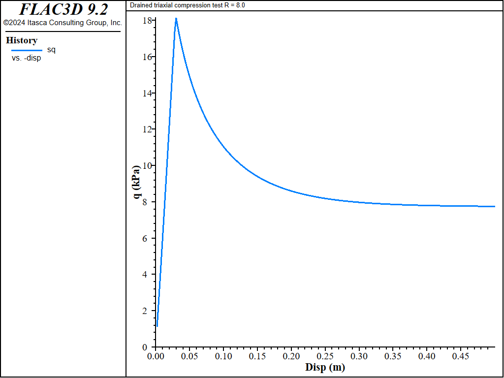
Figure 13: Evolution of deviator stress with axial strain for R = 8—drained test.
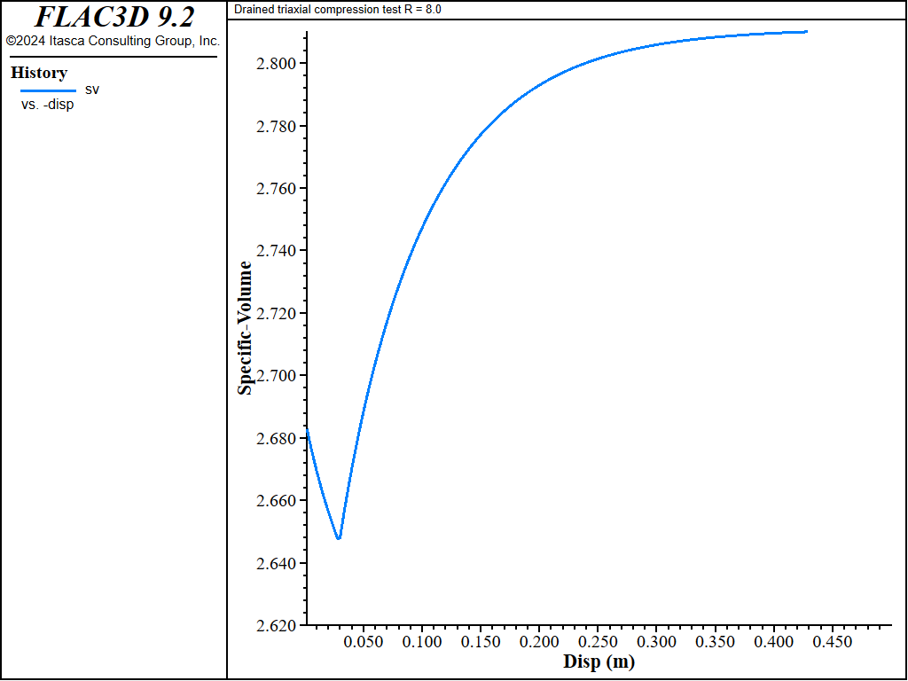
Figure 14: Evolution of specific volume with axial strain for R = 8—drained test.
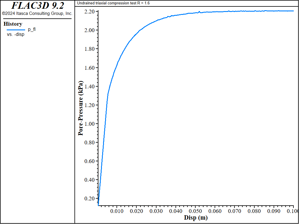
Figure 15: Evolution of pore pressure with axial strain for R = 1.6—undrained test.
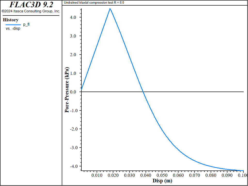
Figure 16: Evolution of pore pressure with axial strain for R = 8—undrained test.
References
Wood, D. M. Soil Behaviour and Critical State Soil Mechanics. Cambridge: Cambridge University Press (1990).
Data Files
TriaxialCompressionTest.dat
; Primary driver for the cam-clay verification problem
;
model new
fish automatic-create off
[global pre_pres = 8]
model title "Drained triaxial compression test R = 1.6"
program call 'drained'
model save 'draineda'
;
model new
fish automatic-create off
[global pre_pres = 40]
model title "Drained triaxial compression test R = 8.0"
program call 'drained'
model save 'drainedb'
;
model new
fish automatic-create off
[global pre_pres = 8]
model title "Undrained triaxial compression test R = 1.6"
program call 'undrained'
model save 'undraineda'
;
model new
fish automatic-create off
[global pre_pres = 40]
model title "Undrained triaxial compression test R = 8.0"
program call 'undrained'
model save 'undrainedb'
drained.dat
model large-strain off
;------------------------------------------------------------
; Drained triaxial compression test on Cam-clay sample
;------------------------------------------------------------
zone create brick size 1 1 1
; --- model properties ---
zone cmodel assign modified-cam-clay
zone property shear 250. bulk-maximum 800.
zone property ratio-critical-state 1.02 lambda 0.2 kappa 0.05
zone property pressure-preconsolidation [pre_pres] pressure-reference 1. ...
                       specific-volume-reference 3.32
; --- boundary conditions ---
zone gridpoint fix velocity-z
zone face apply stress-xx -5. range union position-x 0 position-x 1
zone face apply stress-yy -5. range union position-y 0 position-y 1
zone initialize stress xx -5. yy -5. zz -5.
; FISH to initialize effective pressure property
; This is overkill for a one zone problem, but an example for a larger one.
fish operator initialize(zone)
    zone.prop(zone,'pressure-effective') = ...
        -tensor.trace(zone.stress(zone))/3.0 - zone.pp(zone)
end
[initialize(::zone.list)]
; ... velocity boundary conditions ...
zone gridpoint initialize velocity-z -0.5e-4 range position-z 1.0
; Set up global FISH functions,
; to take histories of values derived from properties
fish define sqcr ; pressure-effective * ratio-critical-state
    local zone = zone.head
    sqcr = zone.prop(zone,'pressure-effective') * ...
           zone.prop(zone,'ratio-critical-state')
end
; --- histories ---
history interval 40
zone history name 'sp' property name 'pressure-effective' zoneid 1
zone history name 'sq' property name 'stress-deviatoric' zoneid 1
fish history name 'sqcr' [sqcr]
zone history name 'sv'   property name 'specific-volume' zoneid 1
zone history name 'disp' displacement-z position (0,0,1)
; Store starting values of some properties -
; used later for analytical comparison
[global pr0 = zone.prop(zone.head,'pressure-reference')]
[global ratio0 = zone.prop(zone.head,'ratio-critical-state')]
[global sv0 = zone.prop(zone.head,'specific-volume-reference')]
[global lambda0 = zone.prop(zone.head,'lambda')]
[global kappa0 = zone.prop(zone.head,'kappa')]
; --- test ---
model cycle 10000
undrained.dat
model large-strain off
;------------------------------------------------------------
; Undrained triaxial compression test on Cam-clay sample
;------------------------------------------------------------
zone create brick size 1 1 1
; --- mechanical properties ---
zone cmodel assign modified-cam-clay
zone property shear 250. bulk-maximum 800.
zone property ratio-critical-state 1.02 lambda 0.2 kappa 0.05
zone property pressure-preconsolidation [pre_pres] pressure-reference 1. ...
                       specific-volume-reference 3.32
; --- boundary conditions ---
zone gridpoint fix velocity-z
zone face apply stress-xx -5. range union position-x 0 position-x 1
zone face apply stress-yy -5. range union position-y 0 position-y 1
zone initialize stress xx -5. yy -5. zz -5.
; FISH to initialize effective pressure property
; This is overkill for a one zone problem, but an example for a larger one.
fish operator initialize(zone)
    zone.prop(zone,'pressure-effective') = ...
        -tensor.trace(zone.stress(zone))/3.0 - zone.pp(zone)
end
[initialize(::zone.list)]
; --- fish functions ---
; ... velocity boundary conditions ...
fish define cycle ; 20 steps on, 20 steps off
    cycle = 1.0 - float(((global.step-1) // 20) % 2)
end
zone face apply velocity-z -0.5e-6 fish cycle range position-z 1.0
; Set up global FISH functions,
; to take histories of values derived from properties
fish define sqcr ; pressure-effective * ratio-critical-state
    local zone = zone.find(1)
    sqcr = zone.prop(zone,'pressure-effective') * ...
           zone.prop(zone,'ratio-critical-state')
end
; --- histories ---
history interval 2000
zone history name 'sp' property name 'pressure-effective' zoneid 1
zone history name 'sq' property name 'stress-deviatoric' zoneid 1
fish history name 'sqcr' sqcr
zone history name 'sv'   property name 'specific-volume' zoneid 1
zone history name 'disp' displacement-z position (0,0,1)
zone history name 'p_fl' pore-pressure zoneid 1
; --- test ---
model cycle 1
fish define bi ; Initialize BIOT modulus
    global v0 = zone.prop(zone.find(1),'specific-volume')
    local n0 = (v0 - 1.) / v0
    bi = 2.e4 / n0
end
model configure fluid-flow
zone fluid property biot-modulus [bi] mobility-coefficient 1e-10
zone fluid property pore-pressure-generation on
zone fluid property effective-cutoff -1e20
; Store starting values of some properties -
; used later for analytical comparison
[global pp0 = zone.prop(zone.find(1),'pressure-preconsolidation')]
[global kappa0 = zone.prop(zone.find(1),'kappa')]
[global lambda0 = zone.prop(zone.find(1),'lambda')]
[global ratio0 = zone.prop(zone.find(1),'ratio-critical-state')]
; Solve
model solve-static cycles 400000
Endnote
| Was this helpful? ... | Itasca Software © 2024, Itasca | Updated: Dec 05, 2024 |
