Hopper Discharge
Introduction
Note
The project file for this example may be viewed/run in PFC.[1] The data files used are shown at the end of this example.
Steps to perform a hopper discharge simulation are presented. The discussion focuses on the PFC3D model but also applies to PFC2D. Figures of both models are shown. This tutorial remains intentionally simple; a more advanced example is discussed in the hopper flow example application, where the influence of filling height and friction on the discharge rate are investigated.
Numerical Model
The hopper geometries, in 2D and 3D, are shown below.
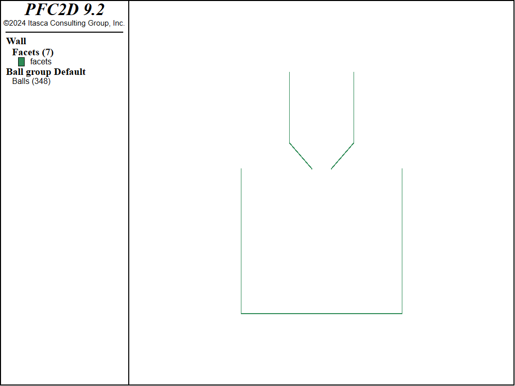
Figure 1: 2D hopper geometry.
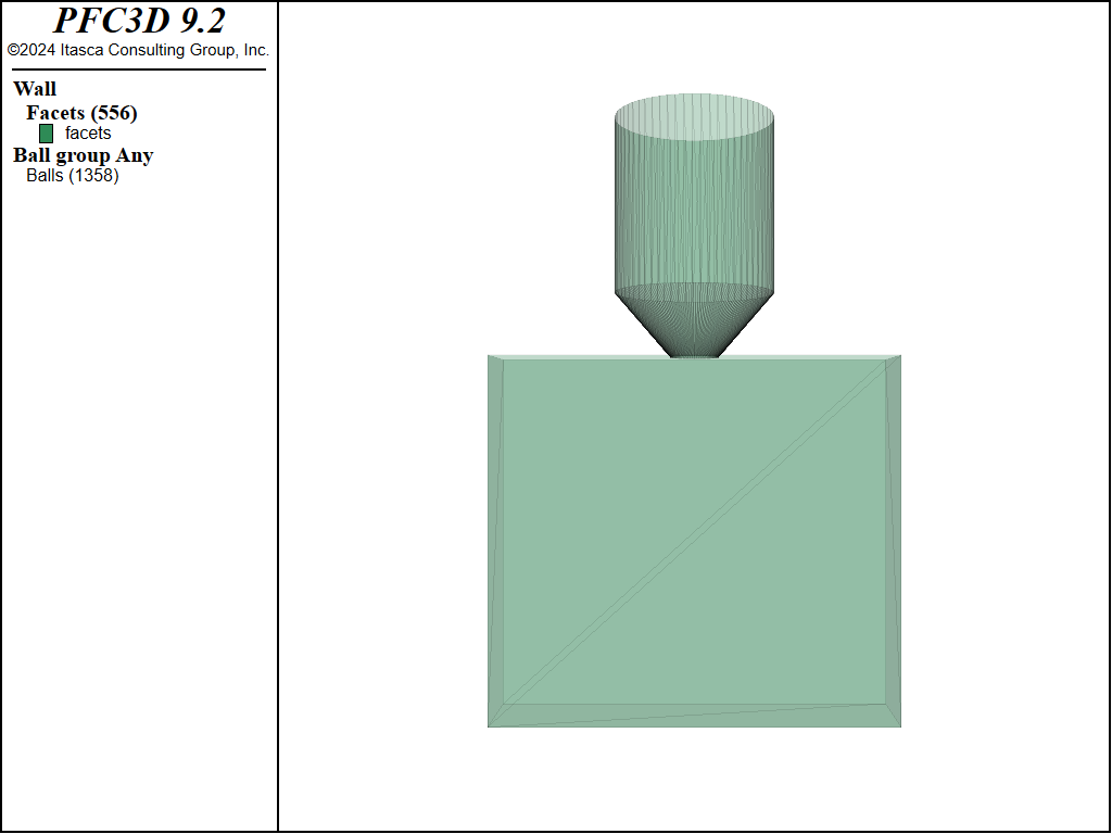
Figure 2: 3D hopper geometries.
The FISH function geometry specifies the dimensions of the hopper. The domain is created according to those dimensions, and the domain conditions are set to destroy balls that move outside the domain extent (refer to the model domain command for details).
The hopper geometry is created using the wall generate command to create conic and cylindrical walls.
For the cylinder, the center position of the bottom face, the radius and the height are required. The cap keyword, which controls whether the cylinder ends are closed, is set to false for both ends. The height and the minimum and maximum radii of the conic frustum top and bottom faces are specified. A minimum radius of 0 generates a cone. For the cone, the cap keyword is set so that the bottom end of the cone is capped but the top remains open.
The default slots of the Contact Model Assignment Table (CMAT) are set for ball-ball and ball-facet contact types. Both slots are filled with the linear contact model but with different properties. Normal viscous damping exists for both ball-ball and ball-facet contacts.
A cloud of overlapping balls is created above the hopper. The density and local damping coefficients of the balls are set using the ball attribute command. Local damping is temporarily set to a large value so that the balls will settle more quickly into the hopper.
The model mechanical timestep scale command is issued to initially activate density scaling in order to quickly reach an initial equilibrium. Gravity is initialized and the model is solved to a target average ratio of 1e-3 with the model solve command.
Note the initial use of the model cycle command with calm keyword, to remove the kinetic energy due to the large overlaps arising from the use of the ball distribute command. In this case, every 50 cycles, both the translational and rotational ball velocities are set to 0.
Six groups of balls are created according to the balls’ initial heights. This is useful for evaluating the flow patterns during hopper discharge. The ball plot item is colored by the textual value group in order to visualize this assignment. A rectangular box is generated to collect the balls flowing from the hopper, and the top of the box is removed.
The following figures show the equilibrated balls in the hoppers prior to discharge.
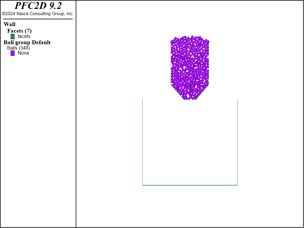
Figure 3: 2D system before discharge.
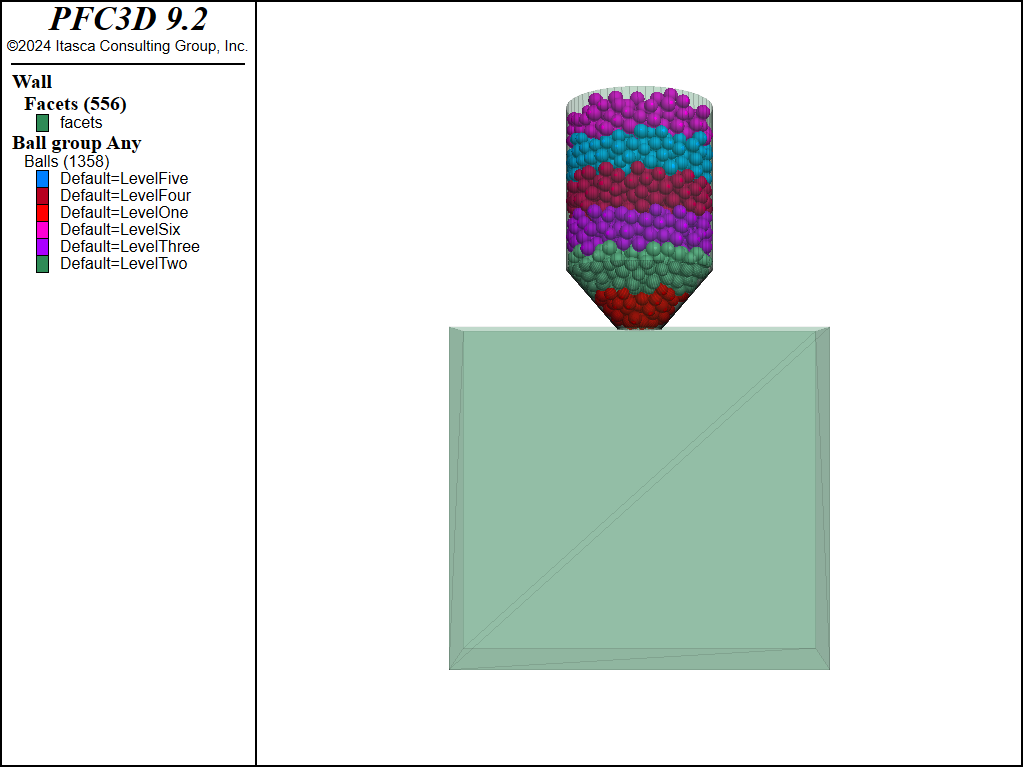
Figure 4: 3D system before discharge.
Before discharging particles from the hopper, the local damping is set to 0, the timestep calculation mode is set to auto (see the model mechanical timestep command), and the mechanical age is reset. The model is then solved to a target time. Snapshots of the systems during discharge are presented below.
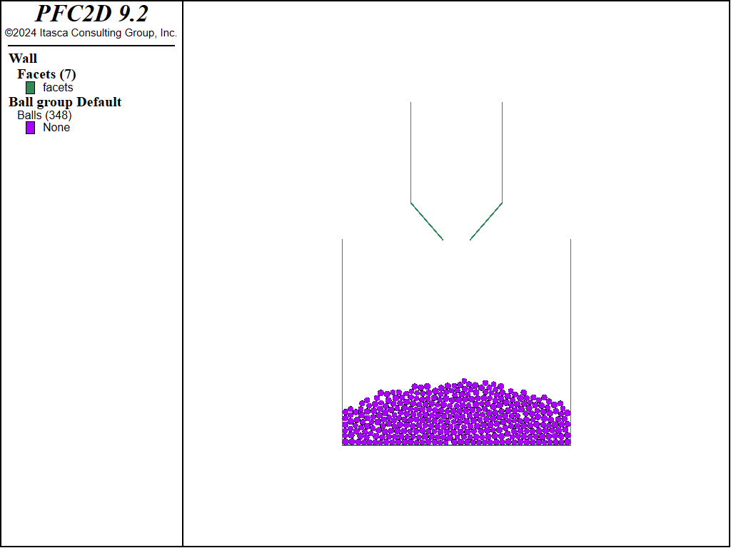
Figure 5: Snapshot of the 2D system during discharge.
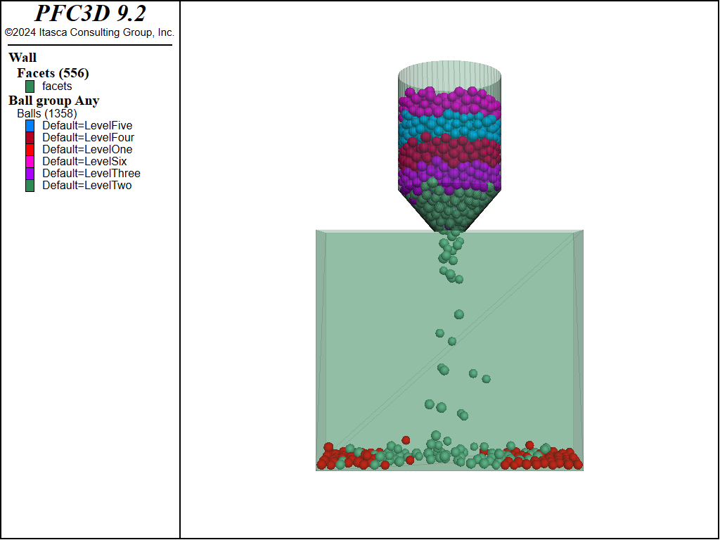
Figure 6: Snapshot of the 3D system during discharge.
Note the use of the ball results command before discharging the balls. The result logic provides the ability to periodically record reduced model states for post-processing purposes. These reduced states can either be saved in memory or output as binary files. In this example, in addition to the ball positions/radii, their group identifiers and velocities are recorded. The makeMovie function (see below) may be executed after the simulation is complete to sequentially load the ball results and export the plot views to bitmap files. Plot view settings (see the c plot commands) are modified as well to move the camera position. A third-party tool may then be used to produce a movie of the hopper discharge based on the exported bitmaps.
Discussion
This tutorial demonstrates the creation of a simple hopper geometry with the wall generate command. This command can generate several simple wall geometries. The hopper is filled and the balls are equilibrated using the model mechanical timestep scale command. Groups are subsequently defined and the balls are allowed to flow from the hopper. The post-processing visualization of dynamic problems like this one can be greatly facilitated by the result logic for balls (ball results), clumps (clump results), and walls (wall results).
Data Files
Hopper.dat (3D)
; fname: Hopper.dat (3D)
;=========================================================================
model new
model large-strain on
model title 'Simple hopper discharge model'

fish define geometry
  W = 20.0
  W0 = 6.0
  Theta = 30
  H = 30.0
  A = (W-W0)*math.tan(Theta*math.pi/180)
end
[geometry]

model domain extent ([-W*1.5],[W*1.5]) ([-W*1.5],[W*1.5]) ([-H*2],[H*2])
model domain condition destroy

wall generate id 1 cylinder base (0.0,0.0,[A])           ...
                            height [H-A] radius [W*0.5] ...
                            cap false false one-wall
wall generate id 2 cone radius [W0*0.5] [W*0.5] height [A] cap true false

contact cmat default type ball-ball model linear  ...
     property kn 5e7 ks 5e7 fric 0.577 dp_nratio 0.2

contact cmat default type ball-facet model linear ...
    property kn 1e8 ks 1e8 fric 0.1 dp_nratio 0.2

model random 10001
ball distribute porosity 0.5 box ([-W*0.35],[W*0.35]) ...
                                 ([-W*0.35],[W*0.35]) ...
                                 ([A],[1.8*H]) radius 0.8 1.0
ball attribute density 1000.0 damp 0.7

model gravity 0 0 -9.81
model cycle 1000 calm 50
model mechanical timestep scale
model solve ratio-average 1e-3

ball delete range cylinder end-1 (0.0,0.0,0.0) ...
                           end-2 (0.0,0.0,[H])  ...
                           radius 0.0 [W*0.5] not
ball group 'LevelOne' range position-z 0.0 [H/6]
ball group 'LevelTwo' range position-z [H/6][2*H/6]
ball group 'LevelThree' range position-z [2*H/6][3*H/6]
ball group 'LevelFour' range position-z [3*H/6][4*H/6]
ball group 'LevelFive' range position-z [4*H/6][5*H/6]
ball group 'LevelSix' range position-z [5*H/6][H*2]

wall delete range position-z 0.0 set id 2
wall generate id 200 box ([-W*1.25],[W*1.25]) ...
                         ([-W*0.25],[W*0.25]) ...
                         ([-H*1.5],0.0)
wall delete range set id 201

model save 'initial'

fish define makeMovie(dur,inc,name)
  i = 0
  curv = inc
  dur = dur
  namefile = name
  loop while (curv <= dur)
    i = i + 1
    dist = 150.0/(i*0.01)
    if dist > 150.0
      dist = 150.0
    endif
    local fname = string.build('%1_%2.png',name,i)
    command
      model results import [i]
      ;plot export bitmap filename [fname]
    endcommand
    curv = curv + inc
  endloop
end

ball attribute damp 0.0
model mechanical timestep automatic
model mechanical time-total 0.0
model results interval mechanical 0.04
wall results active on
ball results active true add-attribute velocity
model solve time 15.0
model save 'final'
;[makeMovie(15,0.04,'test')]

program return
;=========================================================================
; eof: Hopper.dat (3D)
Hopper.dat (2D)
; fname: hopper.dat (2D)
;
; simple hopper discharge tutorial
;=========================================================================
model new
model large-strain on

fish define geometry
  W = 20.0
  W0 = 6.0
  Theta = 30
  H = 30.0
  A = (W-W0)*math.tan(Theta*math.pi/180)
end
[geometry]

model domain extent ([-W*1.5],[W*1.5])([-H*2],[H*2.5])
model domain condition destroy

wall create id 1 vertices ([-W0*0.5],0.0) ([-W*0.5],[A])
wall create id 2 vertices ([W0*0.5],0.0) ([W*0.5],[A])
wall create id 3 vertices ([-W0*0.5],0.0) ([W0*0.5],0.0)
wall create id 4 vertices ([-W*0.5],[A]) ([-W*0.5],[H])
wall create id 5 vertices ([W*0.5],[A]) ([W*0.5],[H])

contact cmat default type ball-ball model linear ...
    property kn 1e7 ks 1e7 fric 0.577 dp_nratio 0.3

contact cmat default type ball-facet model linear ...
    property kn 1e8 ks 1e8 fric 0.1  dp_nratio 0.3

model random 10001
ball distribute porosity 0.5 box ([-W*0.5],[W*0.5]) ...
                                 ([A],[2.0*H]) radius 0.6 0.75
ball attribute density 2000
model cycle 1000 calm 50
model cycle 2000
model mechanical timestep scale
model gravity 0 -9.81
ball delete range position-x [W*0.5] 100
ball delete range position-x -100 [-W*0.5]
model solve ratio-average 1e-4
ball delete range position-y -100 0
model orientation-tracking on
model save 'Hopper2D'

ball group 'LevelOne'   range position-y 0.0 [H/6]
ball group 'LevelTwo'   range position-y [H/6][2*H/6]
ball group 'LevelThree' range position-y [2*H/6][3*H/6]
ball group 'LevelFour'  range position-y [3*H/6][4*H/6]
ball group 'LevelFive'  range position-y [4*H/6][5*H/6]
ball group 'LevelSix'   range position-y [5*H/6][H*1.5]

wall generate id 200 box ([-W*1.25],[W*1.25]) ([-H*1.5],0.0)
wall delete range set id 202
wall delete range set id 3

model mechanical time-total 0.0
model results interval mechanical 0.2 warn off
ball results active on add-attribute velocity
wall results active on
model mechanical timestep automatic

fish define replay(name,plot)
  rmap  = map(0,0)
  map.remove(rmap,0)
  command
    model results map rmap
  endcommand
  local rsize = map.size(rmap)
  local rkeys = map.keys(rmap)
  loop foreach local k rkeys
    local iname = map.value(rmap,k)
    local oname = string.build('%1_t%2.png',name,k)
    command
      model results import [iname]
    endcommand
    if plot = true
      command
        plot bitmap plot 'the system' filename [oname]
      endcommand
    endif
  endloop
end

model solve time 25.0

model save 'final'
[replay('test',false)]
;[replay('test',true)]


program return
;=========================================================================
; eof: hopper.dat (2D)
Endnote
| Was this helpful? ... | Itasca Software © 2024, Itasca | Updated: Dec 05, 2024 |
