Sleeved Triaxial Test of a Bonded Material (FLAC3D)
Problem Statement
Note
The project file for this example is available to be viewed/run in FLAC3D.[1] The main data files used are shown at the end of this example. The remaining data files can be found in the project.
This example demonstrates the use of shell-based structural elements to perform a set of sleeved triaxial tests on a bonded-particle model (BPM). A model of this nature could be investigated using PFC alone. However, in that case, a fair amount of FISH would be required for the sleeved wall to mimic the behavior of an elastic membrane. Here, a sleeve is created from a shell and a BPM is synthesized inside the sleeve as seen in Figure 1. As described in detail in the Wall-Zone Coupling Scheme section, PFC walls are slaved to shell-based structural element. Contacts exist between PFC balls and wall facets; the contact forces and moments at each ball-facet contact are used to determine an equivalent force system to apply to the corresponding shell nodes. In this model, the specimen is created with no initial stress for simplicity and the platens are displaced with a constant velocity. Using this example as a basis, one could easily define the failure envelope of a BPM.
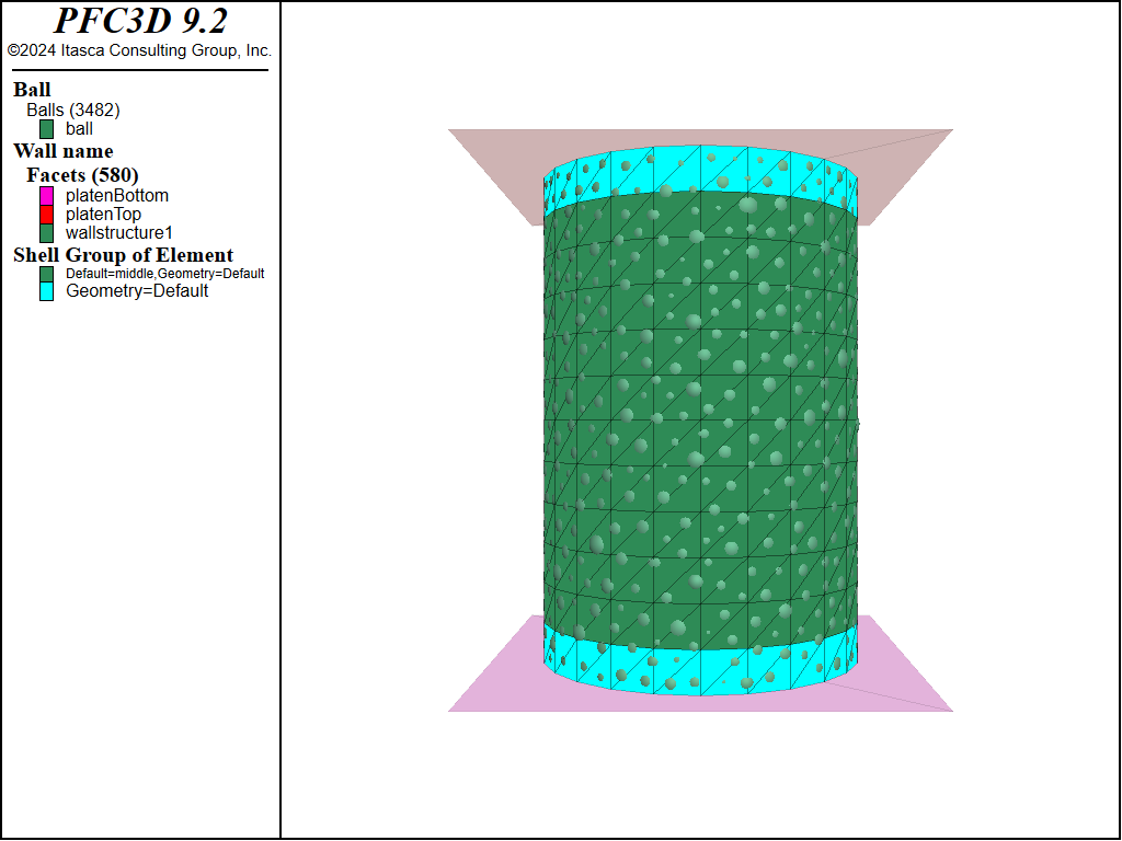
Figure 1: Geometry of the sleeved triaxial test. The BPM is created inside the sleeve.
Coupled PFC-FLAC3D Model
Prior to creating a coupled PFC-FLAC3D model, one must load the PFC modules. These are the DLLs that contain the code responsible for instantiating all PFC related model components. In addition, a set of modules exist to couple PFC walls with FLAC3D zones and shell-based structural elements. By default these modules are not loaded when the FLAC3D application is opened. One may either load these modules via the menu item or with the following commands:
program load module 'contact'
program load module 'pfc'
program load guimodule 'pfc'
program load module 'pfcthermal'
program load guimodule 'pfcthermal'
program load module 'ccfd'
program load guimodule 'ccfd'
program load module 'wallsel'
program load module 'wallzone'
Once a project has been saved with any additional modules loaded, these modules will be loaded whenever the project is opened once again. Note that the additional modules remain loaded until the FLAC3D application is closed.
PFC balls are created within the cylindrical sleeve composed of FLAC3D shells. In order to create
the same initial cloud of balls each time the data files are run, the model random command is used to initialize
the random seed to a specified value. Changing the random seed will result in a different realization of
balls, though statistically, the realizations will be the same. Unlike zones and structural elements,
all PFC model components (i.e., balls, clumps, walls and contacts) can only exist within a user-specified
model domain (see the model domain command). This restriction allows for contact detection and
spatial searching to be simplified and optimized. As PFC always operates in large-strain mode, one
must explicitly activate large-strain mode for zones and structural elements (see the
model large-strain command). PFC, by default, solves the dynamic equations of motion using the
real inertia properties of balls and clumps. In this model, we desire to operate with timestep scaling
in PFC (see the model mechanical command), an approach which is similar to the default FLAC3D
behavior.
With these preliminary steps complete, we dive into creating the initial model.
;define relevant parameters for the cylinder
[rad = 1.0]
[height = 3.0]
[segments = 6]
[halfLen = height/2.0]
[freeRegion = height/2.0*0.8]

;create the cylinder with the geometry logic
;first create arcs making a circle of edges
geometry edge create by-arc origin (0,0,[-halfLen]) ...
   start ([rad*(-1)],0,[-halfLen]) end (0,[rad*(-1)],[-halfLen]) ...
   segments [segments]
geometry edge create by-arc origin (0,0,[-halfLen]) ...
   start (0,[rad*(-1)],[-halfLen]) end ([rad],0,[-halfLen]) ...
   segments [segments]
geometry edge create by-arc origin (0,0,[-halfLen]) ...
   start ([rad],0,[-halfLen]) end (0,[rad],[-halfLen]) ...
   segments [segments]
geometry edge create by-arc origin (0,0,[-halfLen]) ...
   start (0,[rad],[-halfLen]) end ([rad*(-1)],0,[-halfLen]) ...
   segments [segments]
;extrude the edges to make a cylinder
geometry generate from-edges extrude (0,0,[height]) segments [segments*2]
The cylindrical sleeve is created in the geometry logic to be imported as a shell. Arcs are created as geometry edges and extruded vertically to create the cylindrical sleeve. Instead of using the ‘@’ operator, one can use the bracket notation (i.e., ‘[]’) to define FISH variables and to use these values in commands.
With the geometry created, we turn our attention to dealing with the structural elements.
;import the structural elements as a shell from the geometry logic
;and assign groups and properties
structure shell import from-geometry 'Default' element-type dkt-cst
structure node group 'middle' range position-z [-freeRegion] [freeRegion]
structure node group 'top' range position-z [freeRegion] [freeRegion+1]
structure node group 'bot' range position-z [-freeRegion-1] [-freeRegion]
structure shell group 'middle' range position-z [-freeRegion] [freeRegion]
structure shell cmodel assign elastic
structure shell property young 1e6 poisson 0.0 thickness 0.25 density 930.0
;initialize the structural element related data structures
model cycle 0
;In order to use the STRUCTURE APPLY command
;set the local system of each structural
;element to be pointing to the center of the triaxial cell
fish define setLocalSystem
    loop foreach local s struct.node.list()
        local p = struct.node.pos(s)
        local nid = struct.node.id.component(s)
        local mvec = vector(0,0,comp.z(p))
        zdir = math.unit(p-mvec)
        ydir = vector(0,0,1)
        command
            structure node system-local z [zdir] y [ydir] ...
                      range component-id [nid]
        endcommand
    endloop
   command
     structure node fix system-local
   endcommand
end
[setLocalSystem]
;make sure that local damping is active for the structural elements
structure mechanical damping local
;fix the structural element nodes for specimen creation
The structure shell import command is used to create the shell from the created geometry.
Both element and node groups are assigned to simplify boundary condition assignment. The code snippet
also shows a FISH function that is used to set the local axis system of each node as pointing toward
the center of the cylinder so that the structure shell apply command can be used to apply a pressure
on shell elements in the middle of the model. The z- direction points directly to the center of the
cylinder and the y- directions points up. The velocity and rotation of the nodes are fixed so that
balls can be equilibrated inside the sleeve.
Now it is time to create the walls for both the sleeve and the platens.
;create a wall representation of the structural element
wall-structure create
;parameter to set the platen width relative to the cylinder radius
[rad2 = rad*1.3]
;create the platens
wall generate name 'platenTop' polygon ([-rad2],[-rad2],[halfLen]) ...
                                       ([rad2],[-rad2],[halfLen])  ...
                                       ([rad2],[rad2],[halfLen])   ...
                                       ([-rad2],[rad2],[halfLen])
wall generate name 'platenBottom' polygon ([-rad2],[-rad2],[-halfLen]) ...
                                          ([rad2],[-rad2],[-halfLen])  ...
                                          ([rad2],[rad2],[-halfLen])   ...
                                          ([-rad2],[rad2],[-halfLen])
;set the wall resolution strategy to full and set the cutoff angle for
;proximity contacts
wall resolution full
The sleeve is created with the wall-structure create command. In this case wall facets are created
for each shell face and the wall facet vertex velocities and positions are slaved to the corresponding
shell nodes. The top and bottom platens are created with the wall generate command and the
wall resolution mode is set to full with the wall resolution command. In general, contacts
exist between PFC balls and wall facets. If the resolution mode is set the none, all contacts
between facets and balls will be delineated and contribute to the force-displacement response of the
balls. When the wall facet sizes are near to the ball sizes, though, this may produce many more contacts
than if the wall was idealized as a perfect surface without facets. The full scheme is used to
mitigate this situation, and the cutoff-angle is used to control the “smoothness” of the wall.
The wall resolution is discussed in detail in the Faceted Walls in PFC topic.
After the walls are created, the BPM is created within the sleeve.
;set the ball modulus and generate a cloud of balls with arbitrary overlap
[ballemod = 1.0e8]
ball distribute box [-rad] [rad] [-rad] [rad] [-halfLen] [halfLen] ...
                porosity 0.3 radius 0.05 0.1 ...
                range cylinder end-1 (0,0,[-halfLen]) end-2 (0,0,[height]) ...
                      radius [rad*0.95]

;set the ball attributes
ball attribute density 2600 damp 0.8
;set the default contact behavior -
;the deformability method sets properties of the
;linear portion of the contact model
contact cmat default model linearpbond method deformability ...
                   emod [ballemod] kratio 1.0
;allow the balls to rearrange,
;nulling the linear and angular velocities every 100 cycles
model cycle 1000 calm 100

;provide some friction to kill additional energy
;and apply this to all of the contacts
contact cmat default model linearpbond method deformability ...
                   emod [ballemod] kratio 1.0 property fric 0.3
contact cmat apply
;solve to a small average ratio
model solve ratio-average 1e-8

;bond the ball-ball contacts
contact method bond gap 1.0e-2 range contact type 'ball-ball'
;change the existing contact properties
;so that the linear force is incremental and
;supply strength
contact property lin_mode 1 lin_force 0 0 0 pb_ten 2e5 pb_coh 2e6
;set the stiffness of the parallel-bond portion of the contact model
contact method pb_deformability emod [ballemod] kratio 1.0 ...
        range contact type 'ball-ball'

;this set of operations removes all ball velocities
;and all contact forces in the model
;so that the specimen is completely stress free and bonded
model calm
ball fix velocity spin
model cycle 2
ball free velocity spin

;free the nodes in the middle section of the sleeve
;while keeping the top and bottom edges fixed
PFC balls and clumps can either be created without initial overlap or with arbitrary initial overlap.
In this case, the ball distribute command is used to create a cloud of balls with arbitrary
overlaps to a specified volume fraction within a parallelepiped volume. Ball attributes are then assigned
and the contact cmat command is used to specify the contact model behavior. With these steps taken
the balls can be allowed to rearrange. The calm keyword in the model cycle command is
used to periodically remove all kinetic energy from the system. Subsequently the contact cmat
command is given to modify the Contact Model Assignment Table and this change is applied to all contacts.
Some friction is supplied to remove additional energy from the system of balls is cycled to a small
average ratio. The contact method bond command is given to create the BPM by installing parallel
bonds at all ball-ball contacts with gap less than or equal to the specified value. A contact method
is a set of operations that operate to perform a task on contacts, possibly modifying multiple contact
properties. After the bonds have been installed, the parallel bond strength is specified and the normal
force calculation of the linear part of the linear parallel bond contact model
is set to incremental model by specifying lin_mode = 1. This allows one to produce a BPM quickly
without internal stresses. In addition, the stiffnesses of the parallel bond component are set.
By removing all velocities and fixing the ball velocity and spin, all contact forces are nulled after
a few cycles. As a result, the BPM is in equilibrium with no internal stresses. Finally, the shell
nodes in the middle of the sleeve are freed in preparation for the triaxial tests. The initial contacts
of the BPM with no stess are shown in the figure below.
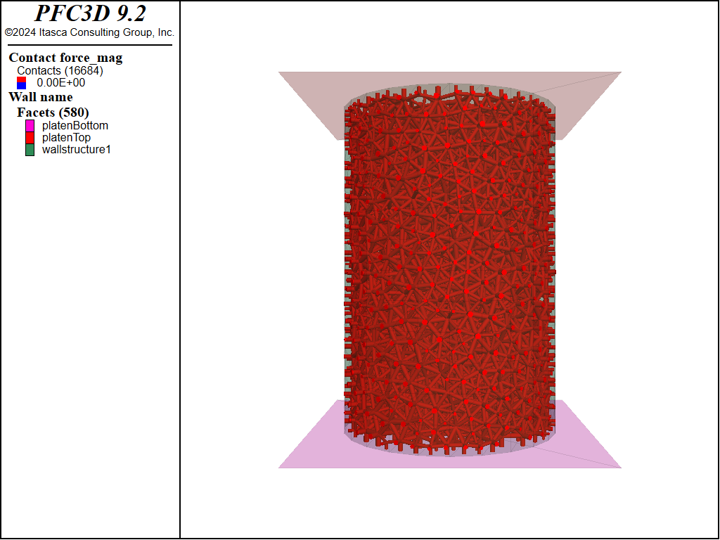
Figure 2: Initial contact forces of the BPM without stress.
With the stress-free BPM created, some additional work is required to build the environment to perform the triaxial tests. The first is a FISH function to calculate the stress and strain based on the platens.
[area = math.pi()*rad^2.0]
;define the stress FISH function to measure the stress and strain
fish define stress
    local topForce = math.abs(comp.z(wall.force.contact(platenTop)))
    local botForce = math.abs(comp.z(wall.force.contact(platenBottom)))
    currentStress = 0.5*(topForce+botForce)/area
    stress = currentStress
    strain = (height - (comp.z(wall.pos(platenTop)) - ...
              comp.z(wall.pos(platenBottom))))/height * 100
    if failureStress <= currentStress
        failureStress = currentStress
        failureStrain = strain
    endif
Here the forces on the platens in the z- direction are used to calculate the average stress on the platens. The strain is also calculated based on the specimen height. The FISH parameters failureStress and failureStrain are used to record the peak stress and strain. This information is used in the FISH function below as a means to terminate cycling.
;define the halt FISH function to stop cycling
;as the platens displace and the material fails
fish define halt
    halt = 0
    if currentStress < failureStress * 0.85
        halt = 1
    endif
Once the current stress level is less than 85% of the maximum stress, cycling will cease. A FISH
function can be used to terminate cycling with the model solve fish-halt command. Once the returned value of the function halt is 1 cycling will terminate.
The following FISH function is used to increase the confining stress on the specimen incrementally:
;define a FISH function to increase the isotropic confining pressure
;in increments so that the bonded material does not break during loading
fish define rampUp(beginIn,ending,increment)
    command
        ball attribute displacement (0,0,0)
        structure node initialize displacement (0,0,0)
    endcommand
    begin = beginIn
    loop while (math.abs(begin) < math.abs(ending))
        begin = begin + increment
        command
            ;apply the confining stress
            structure shell apply [begin] range group 'middle'
            ;apply the same confining stress on the platens
            wall servo force (0,0,[begin*area]) activate true ...
                 range name 'platenTop'
            wall servo force (0,0,[-begin*area]) activate true ...
                 range name 'platenBottom'
            model cycle 200
            model calm
        endcommand
    endloop
    command
        ;once the stress state has been installed cycle and turn off the servo
        ;mechanism on the walls
        model cycle 1000
        wall servo activate false
        wall attribute velocity (0,0,0) range name 'platenTop'
        wall attribute velocity (0,0,0) range name 'platenBottom'
    endcommand
The core of this function is to incrementally increase the confining stress on both the platens and
sleeve. Since we have specified the local system for the shells, it is simple to use the
structure shell apply command to provide confining stress. Also, the built-in wall servo mechanism
is employed, with the wall servo command, to provide stress on the platens. Now it is time to
squeeze some synthetic materials.
Results and Discussion
First the unconfined compression (UCS) test is performed by removing the sleeve and fixing the velocities of the platens. The results of this tests are shown in the figure below. The broken bonds are also shown to demonstrate the pervasive damage of the BPM at failure. Note that the response is quite linear to failure and that the test automatically stopped at 85% of the peak stress. This peak UCS tests of this BPM was 2.20e+06 Pa at 1.13% strain.

Figure 3: Stress-strain response of the BPM to a UCS test along with the broken contact bonds.
To undertake the first triaxial test, the original BPM is loaded and the stress is ramped up from to 1e4 Pa in 1e3 Pa increments. The contacts are show in Figure 4. Notice that the stress is isotropic as the contacts retain nearly their original configuration. One is able to tell this as the contacts are plotted in the force vector direction as opposed to the direction connecting the balls in question.
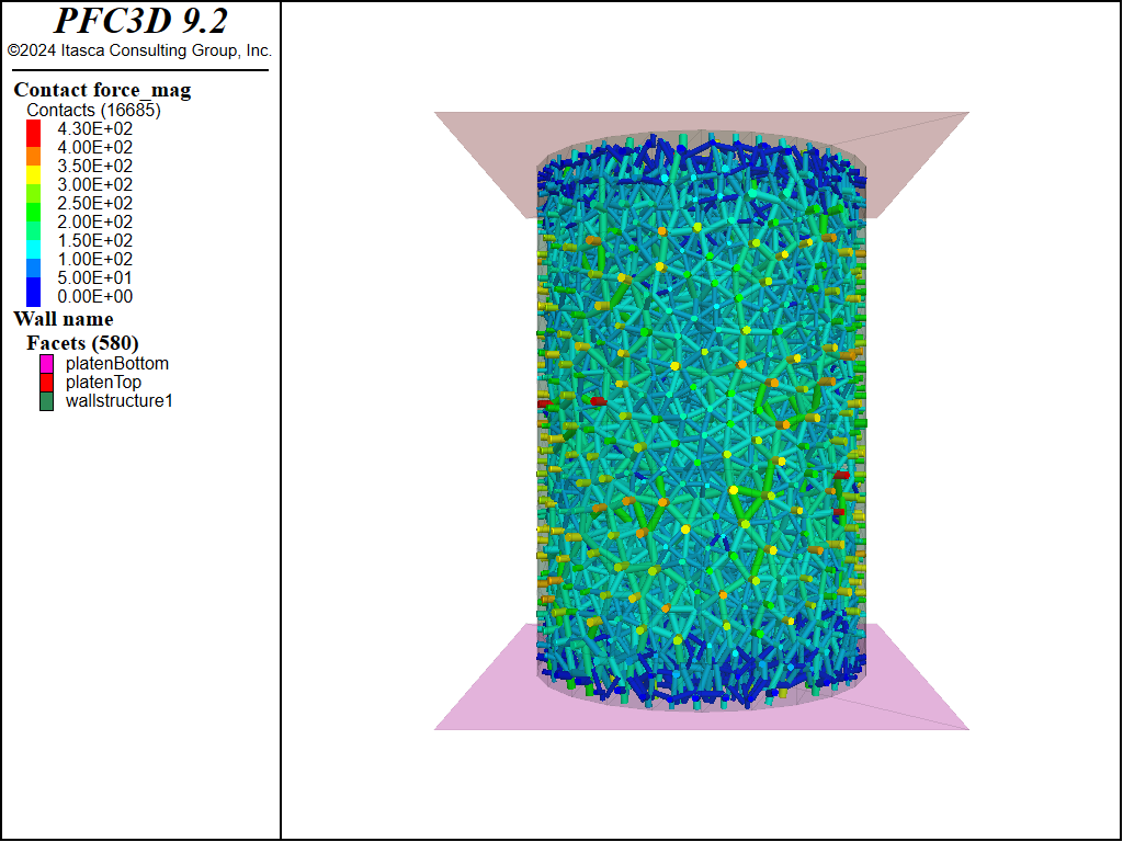
Figure 4: Contact forces oriented in the direction of the force after the stress installation.
The test results with 1e4 Pa confinement are shown in Figure 5. The specimen failed at 1.15% strain with a peak stress of 2.16e+06 Pa. Figure 6 and Figure 7 show the stress-strain responses and broken contact bonds for 5e4 Pa and 1e5 Pa, respectively. The table below presents the peak stress at which the BPM failed for each level of confinement. Notice that, as with real materials, the peak strength increases with confinement. In addition, the stress-strain curves remain linear and similar in slope as with increasing confinement. The slight drop in stress with low confinement can be attributed to using the walls to measure the stress and the relatively small number of balls.
Confinement (Pa) |
Peak Strength (Pa) |
Strain (%) |
|---|---|---|
0 |
2.20e+06 |
1.13 |
1e4 |
2.16e+06 |
1.15 |
5e4 |
2.60e+06 |
1.37 |
1e5 |
2.96e+06 |
1.54 |
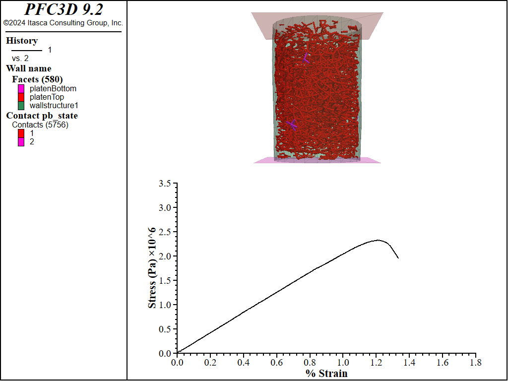
Figure 5: Stress-strain response of the BPM to the triaxial test with 1e4 confinement along with the broken contact bonds.
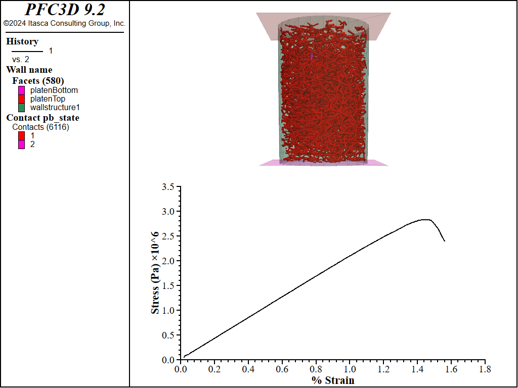
Figure 6: Stress-strain response of the BPM to the triaxial test with 5e4 confinement along with the broken contact bonds.
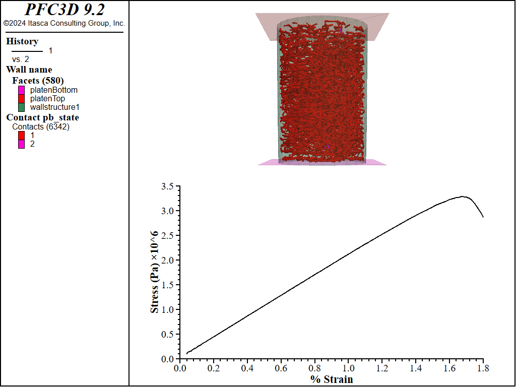
Figure 7: Stress-strain response of the BPM to the triaxial test with 1e5 confinement along with the broken contact bonds.
Taking this example as a starting point, one can effectively delineated the failure envelope of a BPM under realistic triaxial conditions.
Data Files
SleevedTriaxialTest.dat
;-------------------------------------------------------------------
;                Sleeved Triaxial Test of a Bonded
;                Material
;-------------------------------------------------------------------
model new
model title 'Sleeved Triaxial Test of a Bonded Material'
;make repeatable by setting the random number seed
model random 10001
;set the model domain for PFC balls and walls
model domain extent -2 2 condition destroy
;largestrain mode must always be on for coupled simulations
model large-strain on
;apply timestep scaling so the PFC timestep will be 1
model mechanical timestep scale

;define relevant parameters for the cylinder
[rad = 1.0]
[height = 3.0]
[segments = 6]
[halfLen = height/2.0]
[freeRegion = height/2.0*0.8]

;create the cylinder with the geometry logic
;first create arcs making a circle of edges
geometry edge create by-arc origin (0,0,[-halfLen]) ...
   start ([rad*(-1)],0,[-halfLen]) end (0,[rad*(-1)],[-halfLen]) ...
   segments [segments]
geometry edge create by-arc origin (0,0,[-halfLen]) ...
   start (0,[rad*(-1)],[-halfLen]) end ([rad],0,[-halfLen]) ...
   segments [segments]
geometry edge create by-arc origin (0,0,[-halfLen]) ...
   start ([rad],0,[-halfLen]) end (0,[rad],[-halfLen]) ...
   segments [segments]
geometry edge create by-arc origin (0,0,[-halfLen]) ...
   start (0,[rad],[-halfLen]) end ([rad*(-1)],0,[-halfLen]) ...
   segments [segments]
;extrude the edges to make a cylinder
geometry generate from-edges extrude (0,0,[height]) segments [segments*2]

;import the structural elements as a shell from the geometry logic
;and assign groups and properties
structure shell import from-geometry 'Default' element-type dkt-cst
structure node group 'middle' range position-z [-freeRegion] [freeRegion]
structure node group 'top' range position-z [freeRegion] [freeRegion+1]
structure node group 'bot' range position-z [-freeRegion-1] [-freeRegion]
structure shell group 'middle' range position-z [-freeRegion] [freeRegion]
structure shell cmodel assign elastic
structure shell property young 1e6 poisson 0.0 thickness 0.25 density 930.0
;initialize the structural element related data structures
model cycle 0
;In order to use the STRUCTURE APPLY command
;set the local system of each structural
;element to be pointing to the center of the triaxial cell
fish define setLocalSystem
    loop foreach local s struct.node.list()
        local p = struct.node.pos(s)
        local nid = struct.node.id.component(s)
        local mvec = vector(0,0,comp.z(p))
        zdir = math.unit(p-mvec)
        ydir = vector(0,0,1)
        command
            structure node system-local z [zdir] y [ydir] ...
                      range component-id [nid]
        endcommand
    endloop
   command
     structure node fix system-local
   endcommand
end
[setLocalSystem]
;make sure that local damping is active for the structural elements
structure mechanical damping local
;fix the structural element nodes for specimen creation
structure node fix velocity rotation

;create a wall representation of the structural element
wall-structure create
;parameter to set the platen width relative to the cylinder radius
[rad2 = rad*1.3]
;create the platens
wall generate name 'platenTop' polygon ([-rad2],[-rad2],[halfLen]) ...
                                       ([rad2],[-rad2],[halfLen])  ...
                                       ([rad2],[rad2],[halfLen])   ...
                                       ([-rad2],[rad2],[halfLen])
wall generate name 'platenBottom' polygon ([-rad2],[-rad2],[-halfLen]) ...
                                          ([rad2],[-rad2],[-halfLen])  ...
                                          ([rad2],[rad2],[-halfLen])   ...
                                          ([-rad2],[rad2],[-halfLen])
;set the wall resolution strategy to full and set the cutoff angle for
;proximity contacts
wall resolution full
wall attribute cutoff-angle 20

;set the ball modulus and generate a cloud of balls with arbitrary overlap
[ballemod = 1.0e8]
ball distribute box [-rad] [rad] [-rad] [rad] [-halfLen] [halfLen] ...
                porosity 0.3 radius 0.05 0.1 ...
                range cylinder end-1 (0,0,[-halfLen]) end-2 (0,0,[height]) ...
                      radius [rad*0.95]

;set the ball attributes
ball attribute density 2600 damp 0.8
;set the default contact behavior -
;the deformability method sets properties of the
;linear portion of the contact model
contact cmat default model linearpbond method deformability ...
                   emod [ballemod] kratio 1.0
;allow the balls to rearrange,
;nulling the linear and angular velocities every 100 cycles
model cycle 1000 calm 100

;provide some friction to kill additional energy
;and apply this to all of the contacts
contact cmat default model linearpbond method deformability ...
                   emod [ballemod] kratio 1.0 property fric 0.3
contact cmat apply
;solve to a small average ratio
model solve ratio-average 1e-8

;bond the ball-ball contacts
contact method bond gap 1.0e-2 range contact type 'ball-ball'
;change the existing contact properties
;so that the linear force is incremental and
;supply strength
contact property lin_mode 1 lin_force 0 0 0 pb_ten 2e5 pb_coh 2e6
;set the stiffness of the parallel-bond portion of the contact model
contact method pb_deformability emod [ballemod] kratio 1.0 ...
        range contact type 'ball-ball'

;this set of operations removes all ball velocities
;and all contact forces in the model
;so that the specimen is completely stress free and bonded
model calm
ball fix velocity spin
model cycle 2
ball free velocity spin

;free the nodes in the middle section of the sleeve
;while keeping the top and bottom edges fixed
structure node free velocity rotation range group 'middle'

;function for calculating stress and strain as the platens are displaced
;these values will be recorded as a history
;first find the top and bottom platens
[platenTop = wall.find('platenTop')]
[platenBottom = wall.find('platenBottom')]
;define some variables for the calculation
[failureStress = 0]
[currentStress = 0]
[failureStrain = 0]
[area = math.pi()*rad^2.0]
;define the stress FISH function to measure the stress and strain
fish define stress
    local topForce = math.abs(comp.z(wall.force.contact(platenTop)))
    local botForce = math.abs(comp.z(wall.force.contact(platenBottom)))
    currentStress = 0.5*(topForce+botForce)/area
    stress = currentStress
    strain = (height - (comp.z(wall.pos(platenTop)) - ...
              comp.z(wall.pos(platenBottom))))/height * 100
    if failureStress <= currentStress
        failureStress = currentStress
        failureStrain = strain
    endif
end

;define the halt FISH function to stop cycling
;as the platens displace and the material fails
fish define halt
    halt = 0
    if currentStress < failureStress * 0.85
        halt = 1
    endif
end

;define a FISH function to increase the isotropic confining pressure
;in increments so that the bonded material does not break during loading
fish define rampUp(beginIn,ending,increment)
    command
        ball attribute displacement (0,0,0)
        structure node initialize displacement (0,0,0)
    endcommand
    begin = beginIn
    loop while (math.abs(begin) < math.abs(ending))
        begin = begin + increment
        command
            ;apply the confining stress
            structure shell apply [begin] range group 'middle'
            ;apply the same confining stress on the platens
            wall servo force (0,0,[begin*area]) activate true ...
                 range name 'platenTop'
            wall servo force (0,0,[-begin*area]) activate true ...
                 range name 'platenBottom'
            model cycle 200
            model calm
        endcommand
    endloop
    command
        ;once the stress state has been installed cycle and turn off the servo
        ;mechanism on the walls
        model cycle 1000
        wall servo activate false
        wall attribute velocity (0,0,0) range name 'platenTop'
        wall attribute velocity (0,0,0) range name 'platenBottom'
    endcommand
end
;set the platen velocity
[platenVel = 0.000003]

;save the model for future use, including these FISH utility function, before
;any confinement has been applied
model save 'beforeApplication'

;-------------------------------------------------------------------
;test 1: perform a UCS test on the specimen
structure shell delete
wall attribute velocity-z [-platenVel] range name 'platenTop'
wall attribute velocity-z [platenVel] range name 'platenBottom'
ball attribute displacement (0,0,0)
fish history stress
fish history strain
model solve fish-halt halt
model save 'ucs'
[io.out(string(failureStress) + 'Pa ')]
[io.out('at' + string(failureStrain) + '% strain')]

;-------------------------------------------------------------------
;test 2: perform a triaxial test with isotropic confining stress 1e4
model restore 'beforeApplication'
[rampUp(0,-1e4,-1e3)]
model save 'to1e4'
wall attribute velocity-z [-platenVel] range name 'platenTop'
wall attribute velocity-z [platenVel] range name 'platenBottom'
ball attribute displacement (0,0,0)
structure node initialize displacement (0,0,0)
fish history stress
fish history strain
model solve fish-halt halt
model save 'triaxial1e4'
[io.out(string(failureStress) + 'Pa ')]
[io.out('at' + string(failureStrain) + '% strain')]

;-------------------------------------------------------------------
;test 3: perform a triaxial test with isotropic confining stress 5e4
model restore 'to1e4'
[rampUp(-1e4,-5e4,-1e3)]
model save 'to5e4'
wall attribute velocity-z [-platenVel] range name 'platenTop'
wall attribute velocity-z [platenVel] range name 'platenBottom'
ball attribute displacement (0,0,0)
structure node initialize displacement (0,0,0)
fish history stress
fish history strain
model solve fish-halt halt
model save 'triaxial5e4'
[io.out(string(failureStress) + 'Pa ')]
[io.out('at' + string(failureStrain) + '% strain')]

;-------------------------------------------------------------------
;test 4: perform a triaxial test with isotropic confining stress 1e5
model restore 'to5e4'
[rampUp(-5e4,-1e5,-1e3)]
model save 'to1e5'
wall attribute velocity-z [-platenVel] range name 'platenTop'
wall attribute velocity-z [platenVel] range name 'platenBottom'
ball attribute displacement (0,0,0)
structure node initialize displacement (0,0,0)
fish history stress
fish history strain
model solve fish-halt halt
model save 'triaxial1e5'
[io.out(string(failureStress) + 'Pa ')]
[io.out('at' + string(failureStrain) + '% strain')]
Endnote
| Was this helpful? ... | Itasca Software © 2024, Itasca | Updated: Dec 05, 2024 |
