FLAC3D Theory and Background • Constitutive Models

Isotropic Consolidation Test with Modified Cam-Clay Model

Note

To view this project in FLAC3D, use the menu command Help ? Examples…. Choose “ConstitutiveModels/ IsotropicConsolidationModifiedCamClay” and select “IsotropicConsolidationModifiedCamClay.f3dprj” to load. The project’s main data file is shown at the end of this example.

This simple one-zone example exercises the modified Cam-Clay model for a normally consolidated material subjected to several load-unload excursions in an isotropic compression test. Following sentence doesn’t make sense. The initial stresses is at isotropic stress so that \(\sigma_{xx}\) = \(\sigma_{yy}\) = \(\sigma_{zz}\) = -5 kPa. The material properties include the following:

maximum shear modulus (\(G_{max}\))	10 MPa
shear modulus (\(G\))	250 kPa
ratio-critical state (\(M\))	1.02
slope of normal consolidation line (\(\lambda\))	0.2
slope of elastic swelling line (\(\kappa\))	0.05
pressure reference (\(p_1\))	1 kPa
specific volume reference (\(v_{\lambda}\))	3.32
pressure consolidation (\(p_{c0}\))	-5 kPa

The sample is assumed normally isotropic consolidation with \(OCR\) = 1, so the initial mean effective pressure and the preconsolidation pressure are the same. Their values are specified using a simple FISH function:

fish define camclay_ini_p
    loop foreach local p_z zone.list
        local mean_p = -(zone.stress.xx(p_z) + zone.stress.yy(p_z) + zone.stress.zz(p_z))/3.0 - z.pp(p_z)
        zone.prop(p_z,'pressure-effective') = mean_p
        zone.prop(p_z,'pressure-preconsolidation') = mean_p
    endloop
end

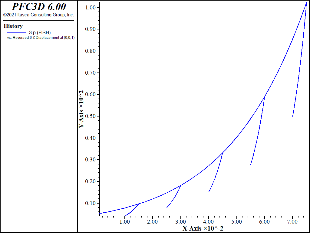
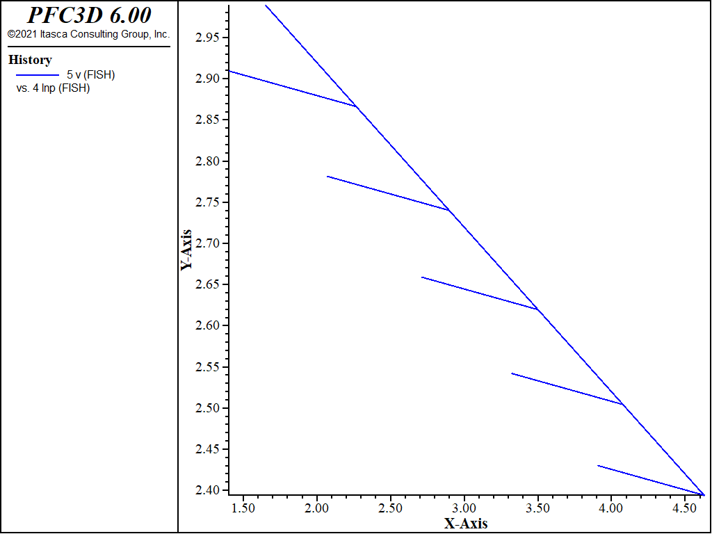
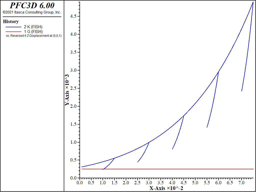
The results are shown in Figure 1, 2, and 3. Figure 1 plots the mean effective pressure history. Figure 2 plots the relation \(v\) vs. \(\ln p\), which shows the normal consolidation line and elastic swelling lines. In this example, the shear modulus is explicitly specified as an input parameter; it is thus assumed constant, while the bulk modulus is changing with the mean effective pressure. The bulk and shear modulus histories are plotted in Figure 3.

Figure 1: Pressure versus displacement.

Figure 2: Specific volume versus \(\ln p\).

Figure 3: Bulk and shear moduli versus displacement.

Data File

;------------------------------------------------------------
; Isotropic compression test on Modified-Cam-clay sample (drained)
;------------------------------------------------------------
model new
model largestrain off
fish automatic-create off
model title "Isotropic compression test for normally consolidated soil"

zone create brick size 1 1 1
zone cmodel assign modified-cam-clay
; --- boundary and initial conditions ---
zone gridpoint fix velocity
zone initialize stress xx -5. yy -5. zz -5.
; --- model properties ---
zone property shear 250. bulk-maximum 10000.
zone property ratio-critical-state 1.02 lambda 0.2 kappa 0.05 
zone property pressure-reference 1. specific-volume-reference 3.32
;
call 'fishfunctions'
@camclay_ini_p
; --- histories ---
history interval 20
fish history @G
fish history @K
fish history @p
fish history @lnp
fish history @v
zone history displacement-z position 0 0 1
; --- test ---
@loadingunloading
model save 'camiso'
return