FLAC3D Theory and Background • Constitutive Models

Oedometer Test with Mohr-Coulomb Model

Note

To view this project in FLAC3D, use the menu command Help ? Examples…. Choose “ConstitutiveModels/ OedometerMohrCoulomb” and select “OedometerMohrCoulomb.f3dprj” to load. The project’s main data file is shown at the end of this example.

This example concerns the determination of stresses in a Mohr-Coulomb material subjected to an oedometer test. In this experiment, two of the principal stress components are equal and, during plastic flow, the stress point evolves along a vertex of the Mohr-Coulomb criterion representation in the \(\Pi\)-plane (the iso-pressure (\(\sigma_{kk}\) = constant) plane in the principal stress space). The purpose is to validate the numerical technique adopted in FLAC3D to handle such a situation. Note that FLAC3D uses no special techniques to deal with yield at vertex points of the Mohr-Coulomb failure locus in the \(\Pi\) plane. Results of a numerical experiment are presented and compared to an exact solution.

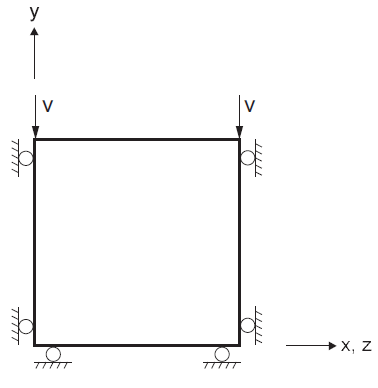
The boundary conditions for the oedometric test are sketched in Figure 1. They correspond to the uniform strain rates

(1)\[\begin{split}\begin{matrix} \Delta {\epsilon}_{11} = 0 \\ \\ \Delta {\epsilon}_{22} = v \Delta t / L \\ \\ \Delta {\epsilon}_{33} = 0 \end{matrix}\end{split}\]

where v is the constant y-component of the velocity applied to the sample \((v < 0)\), and L is the height of the sample.

Assuming zero initial stresses, the principal directions of stresses and strains are those of the coordinate axes. For simplicity, we consider a sample of unit height \(L\) = 1.

Figure 1: Boundary conditions for oedometer test.

In the elastic range, application of Hooke’s law gives, using \({\epsilon}_{22} = v t\) at time \(t\):

(2)\[\begin{split}\begin{matrix} \sigma_{11} = \alpha_2 v t \\ \\ \sigma_{22} = \alpha_1 v t \\ \\ \sigma_{33} = \sigma_{11} \end{matrix}\end{split}\]

where \(\alpha_1 = K + 4/3 G\) and \(\alpha_2 = K - 2/3 G\).

To apply the Mohr-Coulomb failure criterion, we consider the yield functions

(3)\[\begin{split}\begin{matrix} f^1 = {\sigma}_{22} - {\sigma}_{11} N_{\phi} + 2c \sqrt{N_{\phi}} \\ \\ f^2 = {\sigma}_{22} - {\sigma}_{33} N_{\phi} + 2c \sqrt{N_{\phi}} \\ \end{matrix}\end{split}\]

At the onset of yield, \(f^1 = f^2\) = 0 and, using Equations (2) and (3), we find

(4)\[ t = {2c \sqrt{N_{\phi}} \over -v(\alpha_1 - \alpha_2 N_{\phi})}\]

Hence, yielding will only take place provided \(\alpha_1 - \alpha_2 N_{\phi} >\) 0.

During plastic flow, the strain increments are composed of elastic and plastic parts, and we have

(5)\[\begin{split}\begin{matrix} \Delta {\epsilon}_{11} = \Delta {\epsilon}_{11}^e + \Delta {\epsilon}_{11}^p \\ \\ \Delta {\epsilon}_{22} = \Delta {\epsilon}_{22}^e + \Delta {\epsilon}_{22}^p \\ \\ \Delta {\epsilon}_{33} = \Delta {\epsilon}_{33}^e + \Delta {\epsilon}_{33}^p \end{matrix}\end{split}\]

Using the boundary conditions of Equation (1):

(6)\[\begin{split}\begin{matrix} \Delta {\epsilon}_{11}^e = - \Delta {\epsilon}_{11}^p \\ \\ \Delta {\epsilon}_{22}^e = v \Delta t - \Delta {\epsilon}_{22}^p \\ \\ \Delta {\epsilon}_{33}^e = - \Delta {\epsilon}_{33}^p \end{matrix}\end{split}\]

The flow rule for plastic flow along the edge of the Mohr-Coulomb criterion corresponding to \({\sigma}_{11} = {\sigma}_{33}\) has the form (e.g., see Drescher 1991)

(7)\[\begin{split}\begin{matrix} \Delta {\epsilon}_{11}^p = \lambda_1 {\partial g^1 \over \partial {\sigma}_{11}} + \lambda_2 {\partial g^2 \over \partial {\sigma}_{11}} \\ \\ \Delta {\epsilon}_{22}^p = \lambda_1 {\partial g^1 \over \partial {\sigma}_{22}} + \lambda_2 {\partial g^2 \over \partial {\sigma}_{22}} \\ \\ \Delta {\epsilon}_{33}^p = \lambda_1 {\partial g^1 \over \partial {\sigma}_{33}} + \lambda_2 {\partial g^2 \over \partial {\sigma}_{33}} \end{matrix}\end{split}\]

where \(g^1\) and \(g^2\) are the potential functions corresponding to \(f^1\) and \(f^2\):

(8)\[\begin{split}\begin{matrix} g^1 = {\sigma}_{22} - {\sigma}_{11} N_{\psi} \\ \\ g^2 = {\sigma}_{22} - {\sigma}_{33} N_{\psi} \end{matrix}\end{split}\]

After partial differentiation, Equation (7) becomes

(9)\[\begin{split}\begin{matrix} \Delta {\epsilon}_{11}^p = - \lambda_1 N_{\psi} \\ \\ \Delta {\epsilon}_{22}^p = \lambda_1 + \lambda_2 \\ \\ \Delta {\epsilon}_{33}^p = - \lambda_2 N_{\psi} \end{matrix}\end{split}\]

In further considering that by symmetry \(\lambda_1 = \lambda_2\), we obtain

(10)\[\begin{split}\begin{matrix} \Delta {\epsilon}_{11}^p = - \lambda_1 N_{\psi} \\ \\ \Delta {\epsilon}_{22}^p = 2 \lambda_1 \\ \\ \Delta {\epsilon}_{33}^p = - \lambda_1 N_{\psi} \end{matrix}\end{split}\]

The stress increments, derived from Hooke’s law, are given by the relations

(11)\[\begin{split}\begin{matrix} \Delta {\sigma}_{11} = \alpha_1 \Delta {\epsilon}_{11}^e + \alpha_2 (\Delta {\epsilon}_{22}^e + \Delta {\epsilon}_{11}^e) \\ \\ \Delta {\sigma}_{22} = \alpha_1 \Delta {\epsilon}_{22}^e + \alpha_2 2\Delta {\epsilon}_{11}^e \\ \\ \Delta {\sigma}_{33} = \Delta {\sigma}_{11} \end{matrix}\end{split}\]

where we have used the symmetry condition \(\Delta {\epsilon}_{11}^e = \Delta {\epsilon}_{33}^e\).

Substitution of Equation (6) in Equation (11) yields, using Equation (10):

(12)\[\begin{split}\begin{matrix} \Delta {\sigma}_{11} = \alpha_1 \lambda_1 N_{\psi} + \alpha_2 (v \Delta t - 2 \lambda_1 + \lambda_1 N_{\psi}) \\ \\ \Delta {\sigma}_{22} = \alpha_1 (v \Delta t - 2 \lambda_1) + \alpha_2 2 \lambda_1 N_{\psi} \\ \\ \Delta {\sigma}_{33} = \Delta {\sigma}_{11} \end{matrix}\end{split}\]

The parameter \(\lambda_1\) can now be determined by expressing the condition that during plastic flow, \(\Delta f^1\) = 0. Using Equation (3), this condition takes the form

(13)\[ \Delta {\sigma}_{22} - \Delta {\sigma}_{11} N_{\phi} = 0\]

Substitution of Equation (12) in Equation (13) yields, after some manipulations, the expression

(14)\[ \lambda_1 = v \Delta t \lambda\]

where

(15)\[ \lambda = {\alpha_1 - \alpha_2 N_{\phi} \over (\alpha_1 + \alpha_2)N_{\phi} N_{\psi} - 2 \alpha_2(N_{\phi} + N_{\psi}) + 2\alpha_1}\]

The FLAC3D simulation is carried out using a single zone of unit dimensions. Several properties are used in conjunction with the Mohr-Coulomb model:

bulk modulus	200 MPa
shear modulus	200 MPa
cohesion	1 MPa
friction	10°
dilation	10° and 0°
tension	5.67 MPa

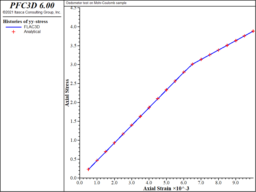
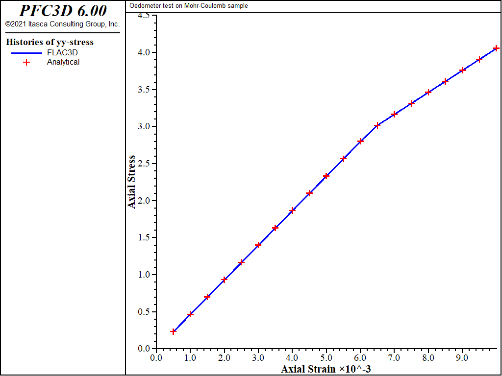
The velocity components are fixed in the x-, y-, and z-directions. A velocity of magnitude 10^-5 m/steps is applied to the top of the model in the negative y-direction for a total of 1000 steps. The stress and displacement components in the y-direction are monitored and compared to the analytic prediction obtained from Equations (2), (4), and (12), using Equations (14) and (15). Two runs are carried out with values of 10° and 0° for the dilation parameter. The match is very good, as can be seen in Figure 2 and Figure 3, where numerical and analytic solutions coincide at the precision of the plot resolution.

Figure 2: Oedometric test—comparison of numerical and analytical predictions for 10° dilation.

Figure 3: Oedometric test—comparison of numerical and analytical predictions for 0° dilation.

Data File

;---------------------------------------------------------------------
; oedometer test
; check plastic flow along an edge of the Mohr-Coulomb criterion
;---------------------------------------------------------------------
model new
model largestrain off
fish automatic-create off
zone create brick size 1 1 1
model title "Oedometer test on Mohr-Coulomb sample"
zone cmodel assign mohr-coulomb
zone property bulk 200 shear 200 co 1 friction 10 tension 5.67 
[global vyv = -1.e-5]
call 'oedometerTheoretical'
zone gridpoint fix velocity
zone gridpoint initialize velocity-y @vyv range position-y 1.0
history interval 50
zone history displacement-y position 0 1 0
fish history @n_sy
fish history @a_sy
model save 'ini'
; --- dilation 10 
zone property dil 10
@d_sigy
model step 1000
model save 'dil10'
; --- dilation 0 
model restore 'ini'
zone property dil 0
@d_sigy
model step 1000
model save 'dil0'