Shallow Foundation

	Tutorial Resources
Data Files	Project: Open {“Footing.p2prj” in PFC2D; “Footing.p3prj” in PFC3D} [1]

Introduction

This tutorial is provided for the new user who wishes to begin experimenting with PFC applied to a geotechnical scenario. The example involves the determination of the bearing capacity of a rough strip footing resting on an assembly of balls.

In this example, a constant vertical velocity is applied to the footing for a fixed duration and the resulting load is monitored. For demonstration purposes, the model is coarse and the ball assembly is limited in spatial extent.

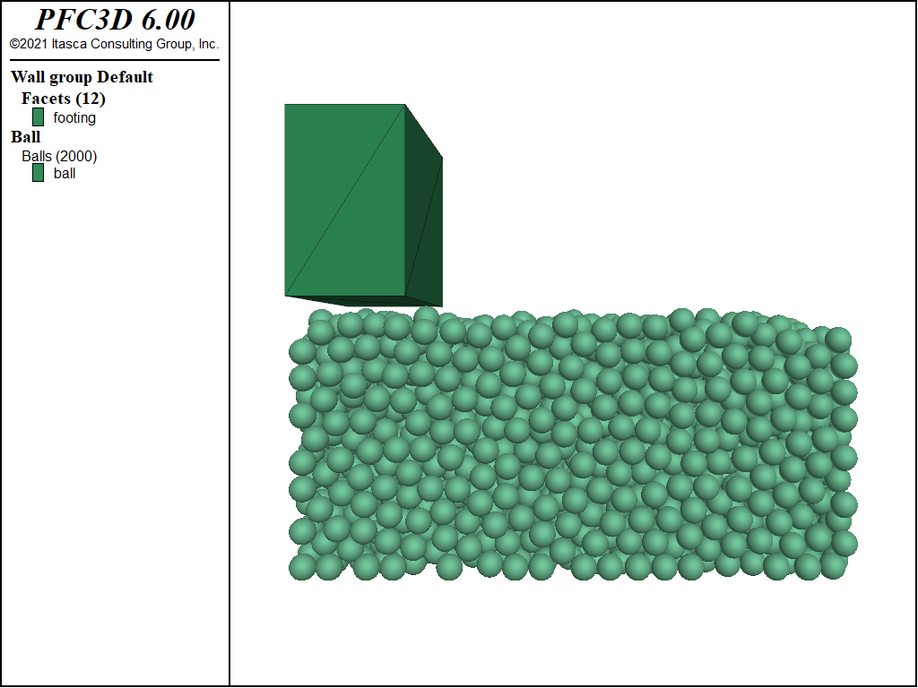
Figure 1: 3D model of a footing over a ball assembly.

In the second stage, the presence of a shallow tunnel in proximity to the foundation is simulated. Two configurations are discussed: with and without the installation of tunnel reinforcement.

Preparation of the Ball Assembly

All of the lines contained in the file “Footing.p3dat” are discussed. The user can also run this problem interactively by typing the commands from the keyboard, pressing Enter at the end of each command line, and seeing the results directly. Additionally, the user can open these data files in the PFC editor, highlight the lines of the data file to be run, and press Ctrl+Shift+E to execute the selected lines of code.

model new
model domain extent (-1,25) (-6,6) (-6,20)
model domain condition destroy

A domain is created, and its dimensions are defined. During the simulation, the balls and walls must stay inside the specified domain. If a ball or wall facet touches the domain, it will be destroyed since the destroy condition is specified (see the model domain command for further details).

wall generate box (0,24) (-5,5) (0,17)
model random 10001
ball generate box (0,24) (-5,5) (0,10) number 2000 radius 0.40   

The wall generate command is used to generate the specimen boundaries. A box is created and its dimensions are specified. Inside this box, a cloud of equally sized balls is generated using the ball generate command. The random seed is set to 10001 prior to eliciting the ball generate command so that the ball positions and radii are identical whenever this model is run.

contact cmat default type ball-ball model linearpbond ...
        property fric 0.577 kn 1e8 ks 1e8             ...
        pb_kn 1e8 pb_ks 1e8 pb_ten 1e6                ...
        pb_coh 1e6 pb_rmul 0.8 dp_nratio 0.2

contact cmat default type ball-facet model linear     ...
        property fric 0.09 kn 1e8 ks 1e8              ...
        dp_nratio 0.2

The Contact Model Assignment Table (CMAT) must be filled in each PFC model for model objects to interact, as each contact is assigned a contact model when created via the CMAT. The default slots of the CMAT are defined for ball-ball and ball-facet contacts. Ball-facet contacts are filled with the linear contact model. The linear parallel bond contact model fills the ball-ball contacts, though. Parallel bonds are installed after the contact method bond is called, once the assembly has reached equilibrium. This action allows for the ball assembly to approximate a solid material.

ball attribute density 2000 radius multiply 1.4

The density attribute of the balls is finally assigned and the ball radii are modified. The ball attribute command assigns mechanical ball attributes (i.e., position, velocity, density, etc.). The ball property command, on the other hand, assigns surface properties that can be used to assign contact model properties (i.e., kn, ks, fric) through the inheritance mechanism. This mechanism is not used in the current model. The ball radii are increased by multiplying the original radii by a factor greater than one (using the multiply keyword).

history interval 5
ball history velocity-z position 12 0 5
model history mechanical unbalanced-maximum

During initial equilibration, the z-velocity of the ball nearest the center of the specimen and the unbalanced force are tracked (see the “History” section). This information can be useful when assessing the stability of the system during a static analysis. These quantities are tabulated every five calculation cycles (see the history interval command).

model mechanical timestep scale
model gravity 0 0 -9.81
model cycle 1000 calm 50
model solve ratio-average 1e-5

Timestep scaling is activated via the model mechanical timestep command with the scale keyword. This logic scales the masses and velocities of the balls to reach an equilibrium configuration quickly. Note that gravitational forces are not affected by timestep scaling, and that the stress path may not be realistic. Subsequent to gravity initialization, a number of calculation steps are done. Note the use of the calm keyword in the model cycle command. This action nulls the translational and rotational velocities of the balls every 50 calculation steps; it is a convenient way to avoid large velocities due to significant overlaps. Finally an equilibrium state is achieved via a model solve to an average ratio of 1e-5.

As shown in Figure 2, the model achieves an equilibrium state relatively quickly.

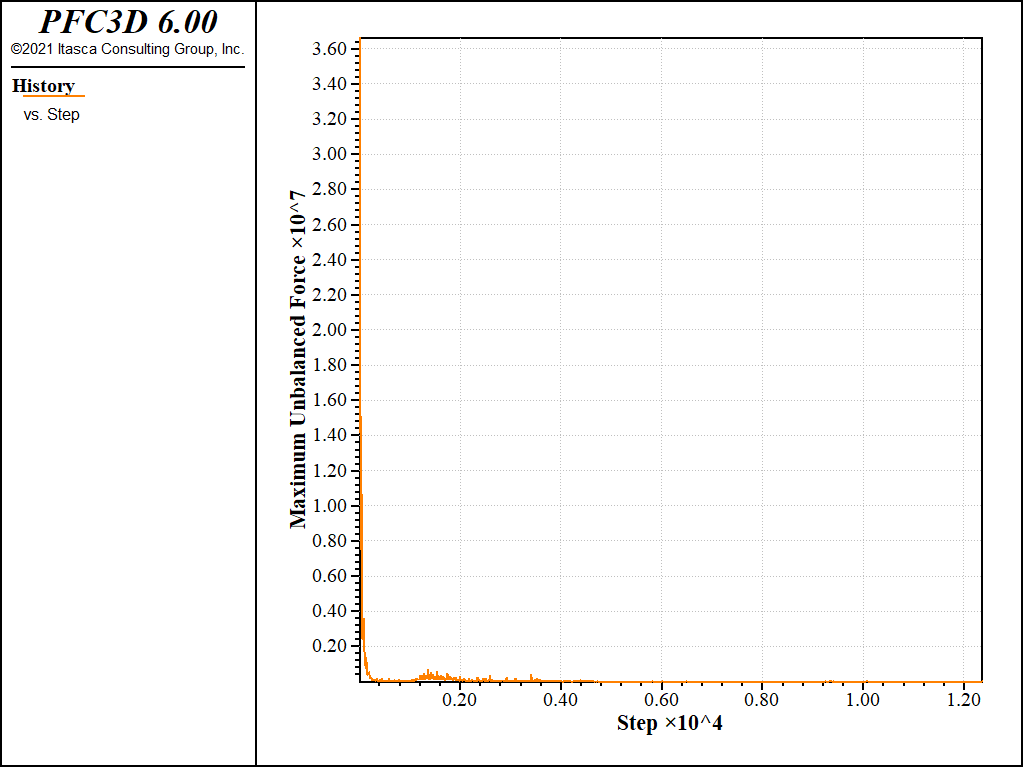
Figure 2: Evolution of the unbalanced force.

wall delete range set id 2
wall generate group 'footing' box (0,5) (-5,5) (12,20) 

The top facets of the box are removed (using the wall delete command). The footing is created above the specimen with the wall generate command. Note that the group keyword is used to assign a group identifier to the newly created facets. The resulting configuration is shown in Figure 1.

contact method bond gap 0.0
model save 'Assembly'

As mentioned above, the contact method bond is used to install parallel bonds in contacts where the gap condition is satisfied. In this case, the upper bound of the gap is 0.0, meaning that parallel bonds are installed at all ball-ball contacts where balls overlap. Had the linear parallel bond model also been applied to ball-facet contacts, parallel bonds would also have been installed in these contacts. Unlike PFC 4.0, balls can be bonded to wall facets in PFC 6.0. The simulation is saved at this point for later use.

Installation of the Foundation

wall attribute velocity-z -0.25 range group 'footing'
history wall force-contact-z id 7
model mechanical timestep auto
model solve time 10.0
wall attribute velocity-z 0.0
model solve ratio-average 1e-5

The vertical velocity of the footing is constant, and the resulting load on the ball assembly is monitored. The vertical contact force is also monitored via a history. The timestep is set to automatic mode since the stress path is important to gauge the loading response; this is a dynamic phenomenon. An additional 10 seconds of model time are simulated using the time solve limit (see the model solve command). Once the foundation has been installed, the wall velocity is nulled and the model is solved to equilibrium once again.

Figure 3 shows the distribution of contact forces in the ball assembly as a consequence of loading.

Figure 3: Distribution of contact forces in the ball assembly after loading.

Excavation of a Shallow Tunnel

The files “Tunnel.p3dat” and “Lining.p3dat” are discussed below. In order to excavate the tunnel from the equilibrated model, one must model restore the model before a number of balls are deleted in a spatial range.

model restore 'Assembly'
ball group 'Tunnel' range cylinder end-1 (16.0,-6.0,6.0) ...
     end-2 (16.0,6.0,6.0) radius 3.0
ball delete range group 'Tunnel'
model cycle 1
model solve ratio-average 1e-5
model save 'StableTunnel'

All of the balls with centers inside the specified cylinder are assigned the group identifier Tunnel and deleted. Alternatively, one could have given the cylindrical range directly in the ball delete command. A single model cycle must be taken, for the contact forces resulting from this change in the model configuration to be accumulated to the balls. (If this cycle is not taken, the subsequent model solve command will stop immediately since the forces applied to the balls by the contacts will be in equilibrium.) The configuration is now stable (see Figure 4) and further experiments can be undertaken.

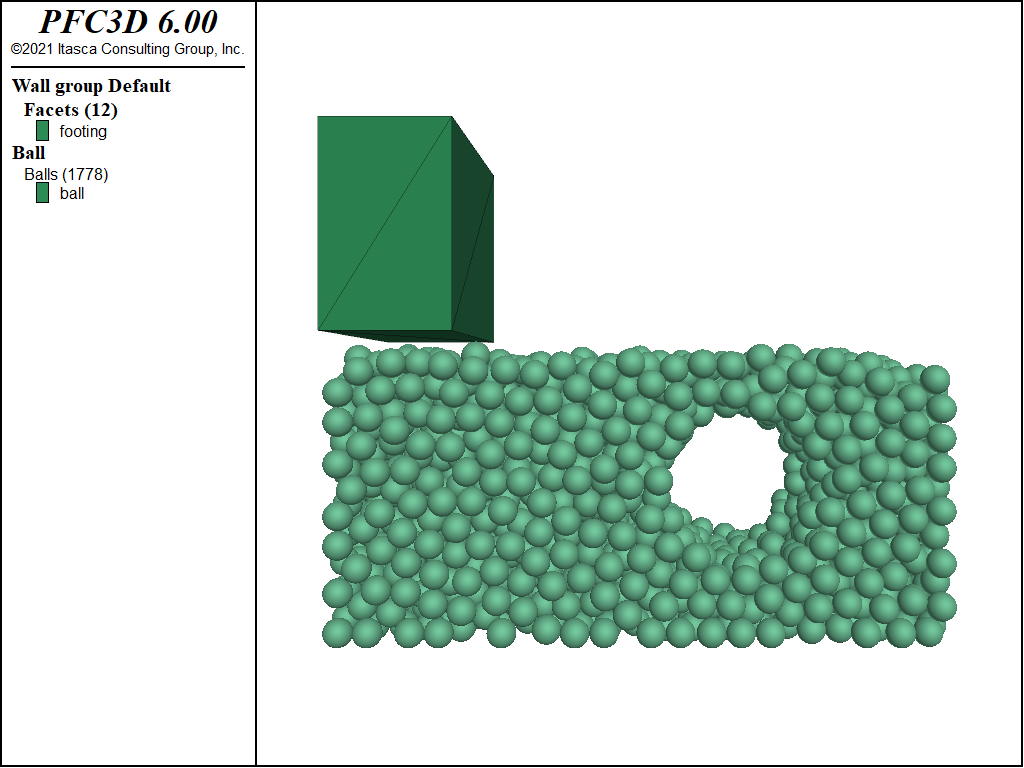
Figure 4: Model configuration with an excavated tunnel.

wall attribute velocity-z -0.25 range group 'footing'
model mechanical timestep auto
model solve time 10.0
wall attribute velocity-z 0.0
model solve ratio-average 1e-5

Application of load from the footing results in catastrophic failure of the unreinforced tunnel. Figure 5 shows the failed configuration.

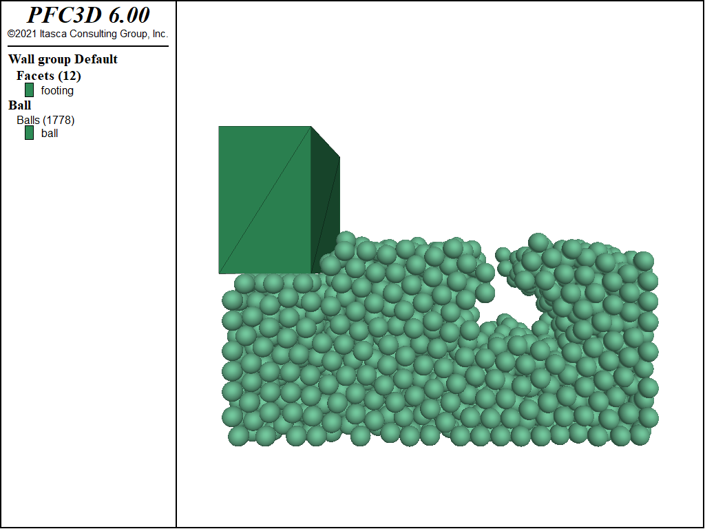
Figure 5: Configuration after installation of the footing near an unreinforced and shallow tunnel.

In the second stage of the simulation, a lining is introduced to reinforce the tunnel.

model restore 'StableTunnel'
contact group 'Lining' range cylinder end-1 (16.0,-6.0,6.0) ...
; A new set of properties is defined for the contacts of the group 'Lining'
contact property fric 0.18 kn 1e8 ks 1e8            ...
        range group 'Lining'

; The assembly is loaded again by the footing. Which differences with respect
; to the case of the unlined tunnel?
model solve time 10.0
; Solve to an equilibrium state again
wall attribute velocity-z 0.0
model save 'LinedTunnel'

; eof: Lining.p3dat

The tunnel lining is simulated by changing the contact properties for those contacts directly adjacent to the excavation. When contacts are assigned group identifiers based on a range, a number of different criteria can be used to decide whether or not the contacts fall within the group. One can specify that a contact falls within a group if either or both of its ends fall within the specified range. Figure 6 shows the effect of this procedure by showing the cohesive strengths of the parallel bonds.

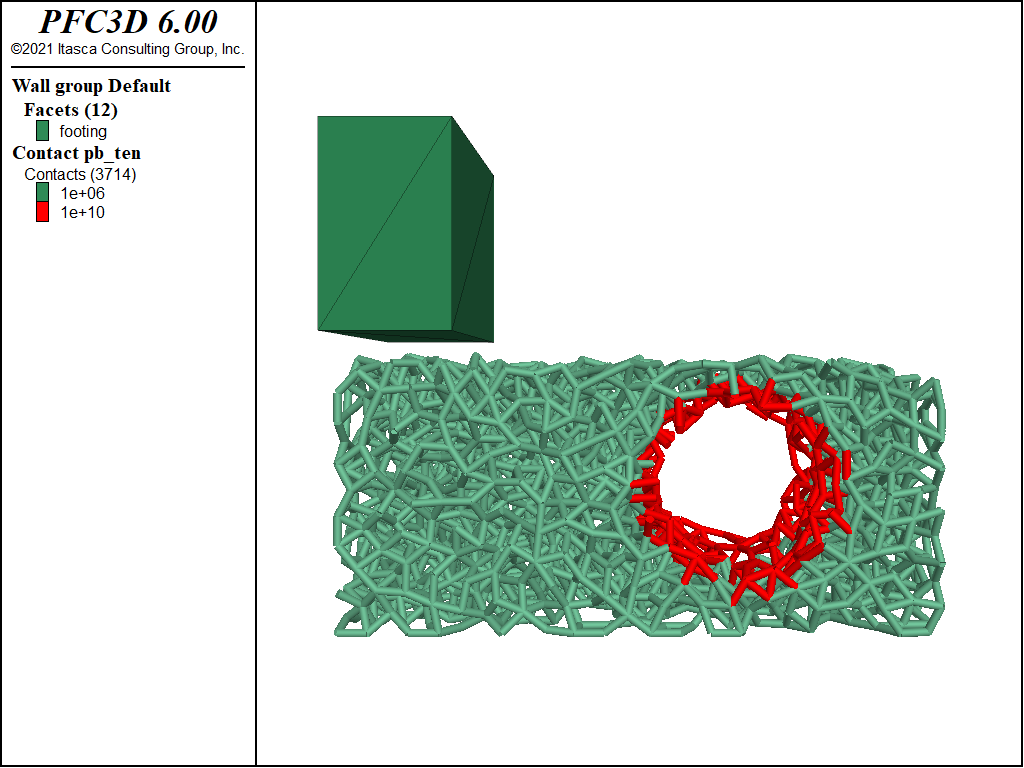
Figure 6: Lining reinforcement for the shallow tunnel.

As with the previous experiments, the footing is given a constant z-velocity for a fixed duration, its velocity is nulled, and the system is solved to equilibrium. Figure 7 shows the result of the reinforcement. The larger cohesive strengths along the tunnel boundary allows the configuration to remain stable in spite of the additional load.

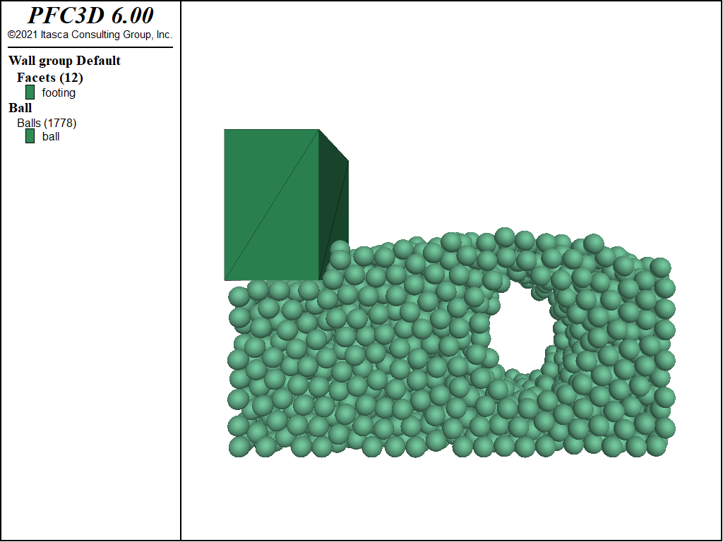
Figure 7: Model configuration after the installation of the footing near a reinforced and shallow tunnel.

Discussion

This simple tutorial illustrates how one might use PFC to investigate a geotechnical problem. An assembly of balls is equilibrated in a box and bonded to make a simple material. A footing is installed to test the stability of three separate configurations: 1) the undisturbed configuration; 2) the configuration with a shallow, unreinforced tunnel; and 3) the configuration with a shallow, reinforced tunnel.

Endnote

[1]

These may be found in PFC3D under the “tutorials/shallow_foundation” folder in the Examples dialog (Help —> Examples on the menu). If this entry does not appear, please copy the application data to a new directory. (Use the menu commands Tools —> Copy App Data …. See the Copy Application Data section for details.)