Adhesive Rolling Resistance Linear Contact Model: Repose Angle

	Problem Resources
Data Files	Project: Open “ReposeAngle.p2prj” in PFC2D or “ReposeAngle.p3prj” in PFC3D [1]

Introduction

In this example, a granular heap is formed by lifting a container initially filled with balls at rest under gravity. The adhesive rolling resistance linear contact model is used, and the simulation is performed several times with varying values of the maximum attractive force \((F_0)\) to investigate its effect on the final shape of the heap. It is found that increasing \(F_0\) increases the slope angle of the heap, as expected. The adhesive rolling resistance linear model has an attraction range \((D_0)\) that defines the distance between balls at which the adhesive force becomes non zero. When changing the value of \(D_0\) during a simulation, it is necessary to use the Contact Model Assignment Table (CMAT) to ensure that contacts will be created automatically between balls with a surface gap less than the attraction range, and the steps necessary to achieve this behavior are demonstrated. This example is addressed in PFC2D and PFC3D.

PFC2D Model

Initial State

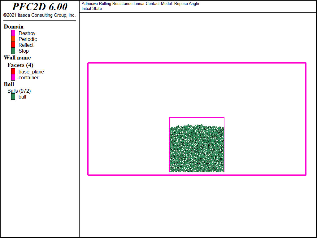
The initial model state consists of a granular column at rest under gravity in a container as shown in Figure 1. This model is created with the data file make_system.p2dat. Selected lines of this file are discussed below.

Figure 1: The initial model state.

For convenience, the input parameters are defined as global FISH variables using inline FISH (see here) with the following lines:

[cyl_height =  100.0e-3]  ; container height     [m]
[ravg       =   1.5e-3 ]  ; ball average radius  [m]
[rdev       =   0.5    ]  ; ball relative radius deviation [-]
[dens       =   2.0e3  ]  ; ball density  [kg/m3]
[poros      =   0.3    ]  ; initial porosity [-]

 ;  contact model properties
[emod   = 1.0e6]  ; Young's modulus (deformability method) [Pa]
[kratio = 2.0  ]  ; stiffness ratio (deformability method) [-]
[fric   = 0.01 ]  ; friction coefficient                   [-]
[dpnr   = 0.2  ]  ; normal critical damping ratio          [-]
[dpsr   = 0.2  ]  ; shear critical damping ratio           [-]
[dpm    = 3    ]  ; dashpot mode                           [-]
[rfric  = 0.0  ]  ; rolling resistance coefficient         [-]
[F0     = 0.0  ]  ; maximum attractive force               [N]
[D0     = 0.0  ]  ; attraction range                       [m]

 ;  Set domain extent and boundary conditions.

The first set of parameters defines the container dimensions, as well as the ball size distribution, density, and the porosity of the cloud of balls that is generated. The container is set to be a 100mm × 100mm square, and the ball radii to have a relative deviation of 0.5 around a mean value of 1.5 mm, with a density of 2000 kg/m³. The geometry is built as two separate walls: a horizontal base plane that spans the entire domain, and a container made of 3 facets.

wall generate id 1 ... 
 name 'base_plane' ... 
 plane

wall create id 100 ... 
 name 'container' ... 
 vertices [-1.0*cyl_rad] 0.0 [-1.0*cyl_rad] @cyl_height ... 
 [-1.0*cyl_rad] @cyl_height [1.0*cyl_rad] @cyl_height ... 
 [1.0*cyl_rad] @cyl_height [1.0*cyl_rad] 0.0

The initial cloud of balls is created using the ball distribute command:

ball distribute porosity @poros ... 
 resolution @ravg ... 
 radius [1.0-0.5*rdev] [1.0+0.5*rdev] ... 
 box [-1.0*cyl_rad] [1.0*cyl_rad] ... 
 0.0 @cyl_height

The second set of parameters defines the contact model properties that will be used in the system. The adhesive rolling resistance linear contact model is assigned to the ball-ball contacts, and the rolling resistance linear contact model is assigned to the ball-wall contacts. There will be no attractive force acting at the ball-wall contacts, and thus, the balls will not stick to the walls.

 ;  stick to the walls.
contact cmat default type ball-ball model arrlinear ... 
 method deformability ... 
 emod @emod ... 
 kratio @kratio ... 
 property fric @fric ... 
 dp_nratio @dpnr ... 
 dp_sratio @dpsr ... 
 dp_mode @dpm ... 
 rr_fric @rfric ... 
 adh_F0 @F0 ... 
 adh_D0 @D0
 
contact cmat default type ball-facet model rrlinear ... 
 method deformability ... 
 emod @emod ... 
 kratio @kratio ... 
 property fric @fric ... 
 dp_nratio @dpnr ... 
 dp_sratio @dpsr ... 
 dp_mode @dpm ... 
 rr_fric @rfric

Please refer to the adhesive rolling resistance linear contact model section for a detailed description of these properties. At this stage, a very low value of the friction coefficient is used, the rolling resistance coefficient is set to zero, and there is no attractive force. These values are used to produce a relatively dense initial state. The contact effective modulus is set to 1 MPa (using the contact model deformability methods). This value is sufficient to ensure that the system remains within the rigid grain limit (i.e., the ratio between the contact effective modulus and the maximal stress at the bottom of the column is large enough, or inversely, the magnitude of the overlaps are small compared to the contacting ball diameters, so that increasing further the contact stiffness would not affect the results) while optimizing the estimated timestep.

Finally, gravity is set as well as the ball density and local damping coefficient attributes; the system is then solved to equilibrium with the following commands:

ball attribute density @dens damp 0.7
model cycle 1000 calm 10
model gravity 9.81
model solve ratio-average 1e-5
ball attribute damp 0.0
model save 'init.p2sav'
program return

Note the use of the calm keyword with the model cycle command to efficiently remove the energy arising from the large initial overlaps inherent to the use of the ball distribute command. Local damping is set to a large value of 0.7 during this phase, as we are only interested in the final equilibrated state, and not in the path followed by the system. It is reset to zero before proceeding to the heap formation.

Heap Formation

The heap is formed by lifting the container wall upwards. This is done using the following set of commands (in the file move_container.p2dat):

 ;  input: fric, rfric, F0, D0
 ; ===========================================================================
[cyl_vel = 5.0e-2]  ; upwards velocity [m/s] 
model mechanical time-total 0.0

 ;  *** Modify Material Properties
 ;  Modify properties of existing ball-ball and ball-facet contacts.
contact property fric @fric rr_fric @rfric adh_f0 @F0 adh_d0 @D0 ... 
 range contact type 'ball-ball'
contact property fric @fric rr_fric @rfric ... 
 range contact type 'ball-facet'
 ;  Modify properties of future ball-ball contacts.
contact cmat default type ball-ball model arrlinear ... 
 method deformability ... 
 emod @emod ... 
 kratio @kratio ... 
 property fric @fric ... 
 dp_nratio @dpnr ... 
 dp_sratio @dpsr ... 
 dp_mode @dpm ... 
 rr_fric @rfric ... 
 adh_f0 @F0 ... 
 adh_d0 @D0
 ;  Modify properties of future ball-facet contacts.
contact cmat default type ball-facet ... 
 property fric @fric rr_fric @rfric
 ;  Proximity has changed automatically from change to a_d0.
 ;  Force creation of new contacts via remapping of cell space.
model clean

wall attribute velocity-y @cyl_vel range id 100 by wall
ball attribute displacement multiply 0.0
model solve time [0.75*cyl_height/cyl_vel]
wall attribute velocity-y 0.0 range id 100 by wall
model solve ratio-average 1e-5
model save ...
 [string.build('final-fric_%1_rfric_%2_F0_%3_D0_%4.p2sav',fric,rfric,F0,D0)]

This file is not intended to be executed directly. Instead, it is invoked sequentially from a Python script in order to perform a series of simulations with different property sets. There are four properties: the friction coefficient (fric), the rolling resistance coefficient (rfric), the maximum attractive force (F0) and the attraction range (D0). These properties are assigned to existing contacts, and to future contacts that may form during subsequent cycling. Values of fric and rfric are assigned to all contacts, while values of F0 and D0 are assigned only to the ball-ball contacts. This provides an example of creating an arrlinear material using the CMAT, which is discussed further at this link.

The four properties are assigned values in the Python script (in the file do_analysis.py):

import itasca
itasca.command("python-reset-state off")

fric_list  = [0.5]
rfric_list = [0.1]
# F0_list is {0, 1, 5} times weight of single particle [N]
# D0_list is 100% of avg. particle radius [m]
F0_list = [0.0,0.14,0.7]
D0_list = [1.5e-3]

for f in fric_list:
  for rf in rfric_list:
    for myF0 in F0_list:
      for myD0 in D0_list:
        itasca.command("""
                         model restore \'init\'
                         [fric  = {0}]
                         [rfric = {1}]
                         [F0    = {2}]
                         [D0    = {3}]
                         program call \'move_container.p2dat\'
                       """.format(f,rf,myF0,myD0)

Four lists are defined, and nested loops are used to assign the particular set of properties for a single model run. For each run, the initial state is restored, the properties are assigned to the four FISH variables, and the move_container.p2dat data file is called. The model runs use the following property values. The friction coefficient and the rolling friction coefficient are held constant at 0.5 and 0.1, respectively. The maximum attractive force is set equal to zero, one and five times the average weight of a single particle (\(W = \rho V g = \rho (\pi R^2 t) g \approx 0.14\) N), and the attraction range is held constant at 100% of the average particle radius.

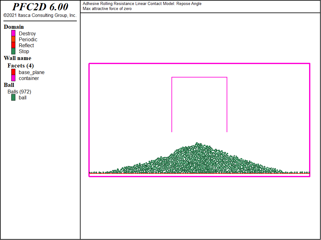
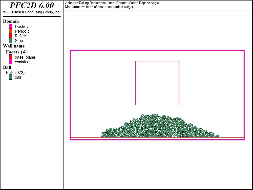
The final states for the three different values of the maximum attractive force \((F_0)\) are shown in Figures 2 to 4. When there is no attractive force, the heap shown in Figure 2 forms. When \(F_0\) is set equal to the average particle weight, the heap becomes more compact with a larger repose angle, because the attractive force is pulling the particles together as shown in Figure 3. When \(F_0\) is increased to five times the average particle weight, the attractive force has become so large that a heap does not form; instead, the particles maintain the container shape as shown in Figure 4. If the attractive force is now set to zero by issuing the following commands (in the file zero_F0.p2dat):

; Zero F0 at existing and future contacts, solve.
model restore 'final-fric_0.5_rfric_0.1_F0_0.7_D0_0.0015.p2sav'

contact property adh_f0 0.0
contact cmat default type ball-ball ...
             property adh_f0 0.0
model cycle 10
model solve ratio-average 1e-5

then the particles can no longer maintain the container shape, and the assembly collapses into the dispersed heap shown in Figure 5.

Figure 2: The final model state with maximum attractive force of zero.

Figure 3: The final model state with maximum attractive force of one times average particle weight.

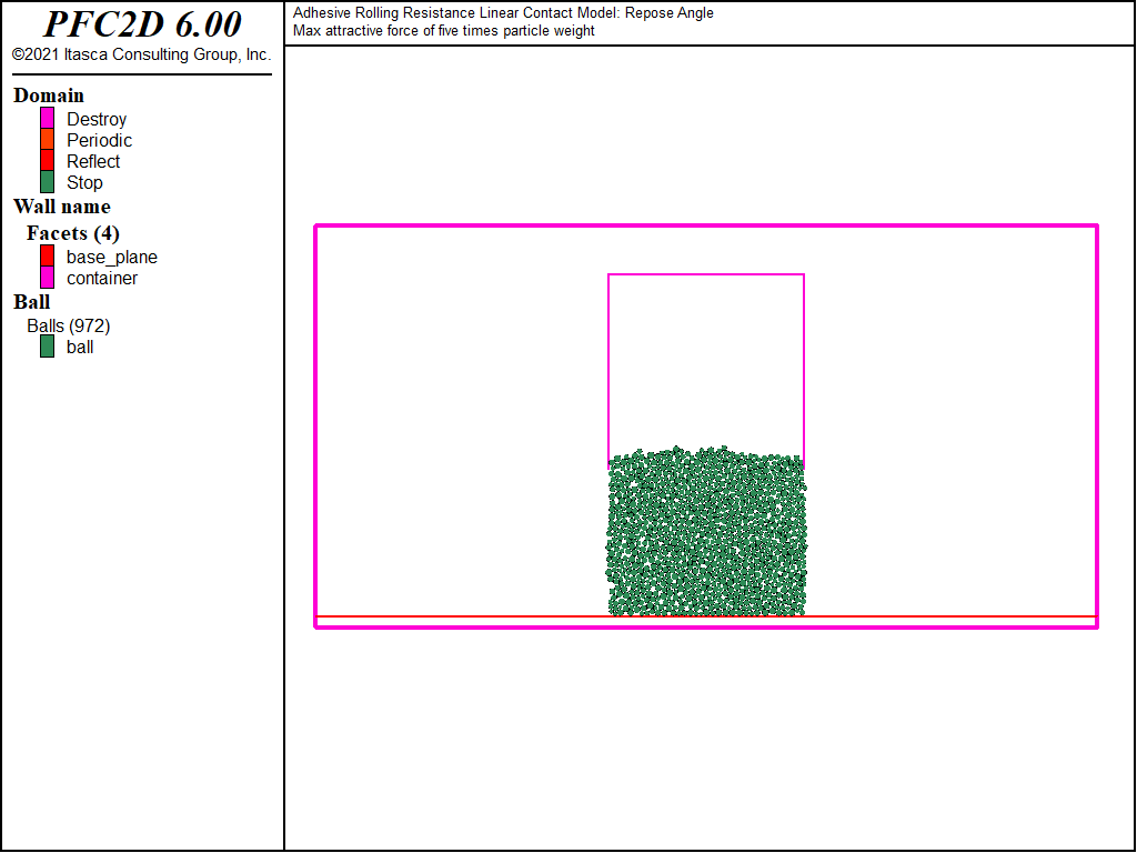
Figure 4: The final model state with maximum attractive force of five times average particle weight.

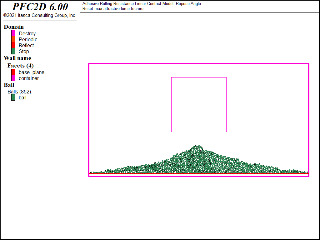
Figure 5: The final model state after setting the maximum attractive force in the system shown in Figure 4 equal to zero.

PFC3D Model

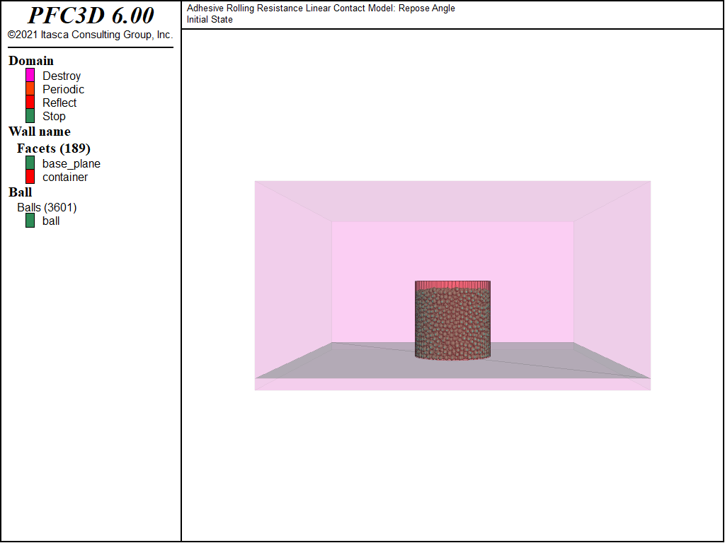
The PFC3D model is similar to the PFC2D model described above, with the difference that the container is a cylinder (with a height and diameter of 100 mm), and the balls have an average radius of 3.0 mm with a relative deviation of 0.25 to limit the size of the model. The initial system is shown in Figure 6. It is constructed using the file make_system.p3dat, and the heap formation is simulated using the file do_analysis.py, which sequentially calls move_container.p3dat to perform multiple runs with different values of the maximum attractive force.

Figure 6: The initial model state.

The model runs use the following property values. The friction coefficient and the rolling friction coefficient are held constant at 0.5 and 0.1, respectively. The maximum attractive force is set equal to zero, one and five times the average weight of a single particle (\(W = \rho V g = \rho ({4\over3} \pi R^3) g \approx 2.2 \times 10^{-3}\) N), and the attraction range is held constant at 5% of the average particle radius.

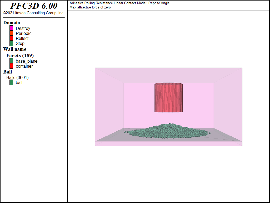
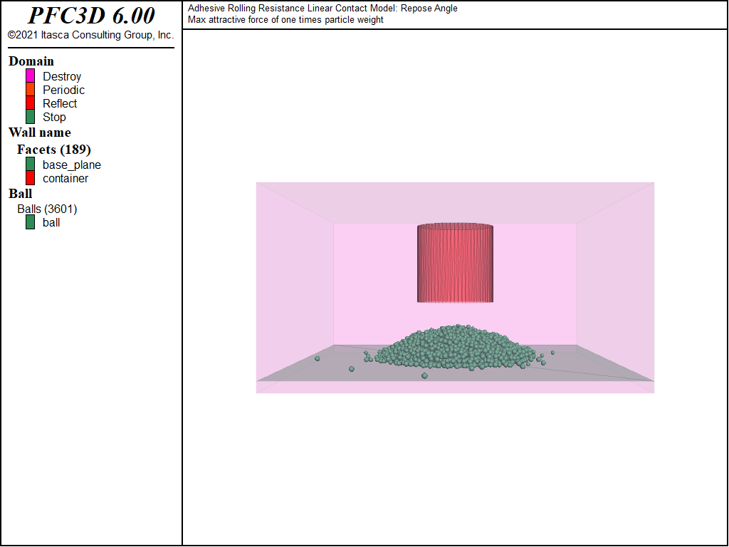
The final states for the three different values of the maximum attractive force \((F_0)\) are shown in Figures 7 to 9. When there is no attractive force, the heap shown in Figure 7 forms. When \(F_0\) is set equal to the average particle weight, the heap becomes more compact with a larger repose angle, because the attractive force is pulling the particles together as shown in Figure 8. When \(F_0\) is increased to five times the average particle weight, the attractive force has become so large that a heap does not form; instead, the particles maintain the container shape as shown in Figure 9. If the attractive force is now set to zero by issuing the following commands (in the file zero_F0.p3dat):

 ;  Zero F0 at existing and future contacts, solve.
model restore 'final-fric_0.5_rfric_0.1_F0_0.011_D0_0.00015.p3sav'

contact property adh_f0 0.0
contact cmat default type ball-ball ... 
           property adh_f0 0.0
model cycle 10
model solve ratio-average 1e-5

then the particles can no longer maintain the container shape, and the assembly collapses into the dispersed heap shown in Figure 10.

Figure 7: The final model state with maximum attractive force of zero.

Figure 8: The final model state with maximum attractive force of one times average particle weight.

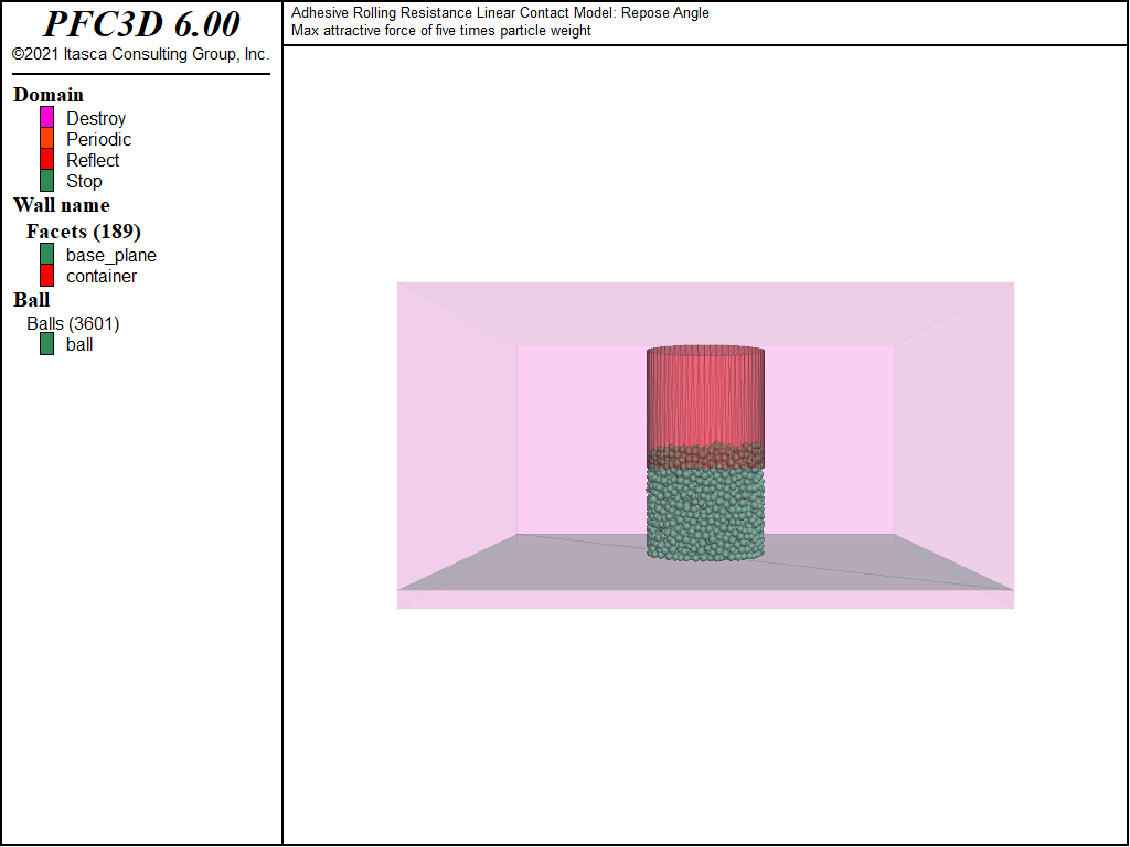
Figure 9: The final model state with maximum attractive force of five times average particle weight.

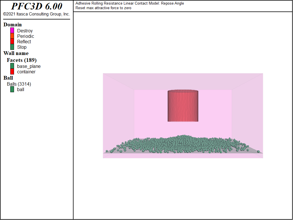
Figure 10: The final model state after setting the maximum attractive force in the system shown in Figure 9 equal to zero.

Discussion

This example exercises the adhesive rolling resistance linear contact model in the situation of a heap formed by moving upwards a container initially filled with balls at rest under the action of gravity, with both PFC2D and PFC3D. The evolution of the shape of the heap with increasing maximum attractive force \((F_0)\) is investigated, and shown to conform to the expected behavior. Increasing \(F_0\) increases the slope angle of the heap, and when \(F_0\) is increased sufficiently, the ball assembly does not form a heap; instead, it maintains the container shape. This example provides qualitative results that are in keeping with the expected behavior.

Endnote

[1]

These files may be found in PFC2D or PFC3D under the “verification_problems/adhesive_rolling_resistance/repose_angle” folder in the Examples dialog (Help —> Examples on the menu). If this entry does not appear, please copy the application data to a new directory. (Use the menu commands Tools —> Copy App Data …. See the “Copy Application Data” section for details.)