Linear Contact Model: Calibrating the Normal Critical Damping Ratio

	Problem Resources
Data File	Project: Open “LinearContactModel.p3prj” in PFC3D [1]

Problem Statement

When viscous damping is used in a PFC model with a linear contact model, an appropriate damping constant should be specified for the simulation to reproduce a realistic response. One way to do this is to calibrate the damping by using the relation between the damping constant and the restitution coefficient. [Kawaguchi1992] derived the relation by solving the equations of motion for free vibration with viscous damping. This derivation is presented. Also, the result of drop tests using PFC3D is compared with the analytical solution.

The linear contact model and its parameters are described in the “Linear Model” section.

The equation of motion for free vibration with viscous damping is given by Equation (1):

(1)\[m \ddot{x} + c\dot{x} + k x = 0\]

where \(m\) is the mass, \(c\) is the damping constant (coefficient of viscous damping), and \(k\) is the stiffness.

Solution of Equation (1) is given by Equation (2):

(2)\[x(t) = C_1 e^{(-\zeta+\sqrt{\zeta^2-1})^{\omega_n t}} + C_2 e^{(-\zeta-\sqrt{\zeta^2-1})^{\omega_n t}}\]

where \(C_1\) and \(C_2\) are arbitrary constants to be determined from the initial conditions. Also, \(\zeta\) is defined as the ratio of the damping constant to the critical damping constant, as given by Equation (3):

(3)\[\zeta = c / c_c\]

where \(c_c\) is the critical damping constant (Equation (4)):

(4)\[c_c = 2m\sqrt{\frac{k}{m}}=2 \sqrt{km} = 2 m \omega_n\]

where \(\omega_n\) is the natural frequency of the system.

This case corresponds to an underdamped system, as shown by the rebound of two impacting objects.

For the initial conditions \(x=x_0,\dot{x}(t=0)=\dot{x}_0\) , the solution for Equation (1) is given by Equation (5):

(5)\[x(t) = e^{-\zeta \omega_n t} \Big( x_0 \cos{\omega_d t} + \frac{\dot{x}_0 + \zeta \omega_n x_0}{\omega_d}\sin{\omega_d t} \Big)\]

where \(\omega_d\) is the frequency of the damped vibration, given by

(6)\[\omega_d = \sqrt{1-\zeta^2 \omega_n}\]

By substituting \(x_0\) = 0 into Equation (5):

(7)\[x(t) = e^{-\zeta \omega_n t} \Big( \frac{\dot{x}_0}{\omega_d}\sin{\omega_d t} \Big)\]

(8)\[\dot{x}(t) = -\zeta \omega_n e^{-\zeta \omega_n t} \Big( \frac{\dot{x}_0}{\omega_d}\sin{\omega_d t} \Big) + e^{-\zeta \omega_n t} \dot{x}_0 \cos{\omega_d t}\]

After half of the time period \(\pi/\omega_d\) (period of oscillation), the system recovers the position at \(x\) = 0. The velocity of the system is given by Equation (9):

(9)\[\dot{x}(t=\frac{\pi}{\omega_d}) = - e^{-\zeta \omega_n \frac{\pi}{\omega_d}} \dot{x}_0\]

Hence, the restitution coefficient \(\alpha\) is given by

(10)\[\alpha = - \frac{\dot{x}(t=\frac{\pi}{\omega_d})}{\dot{x}_0} = e^{-\zeta \omega_n \pi / \omega_d} = e^{-\frac{\zeta \pi}{\sqrt{1-\zeta^2}}}\]

Also, the ratio of the damping constant to the critical damping constant, \(\zeta\), and the damping constant, \(c\), are given by Equation (11) and Equation (12), respectively:

(11)\[\zeta = \frac{\ln(\alpha)}{\sqrt{\ln^2(\alpha)+\pi^2}}\]

(12)\[c = \frac{2\sqrt{km}\ln(\alpha)}{\sqrt{\ln^2(\alpha)+\pi^2}}\]

PFC3D model

A drop test is conducted in which two rows of 16 balls each are dropped under gravity from a one-meter height above a wall surface. The linear contact model is used, with a contact normal stiffness of \(k_n\) = 5.0 × 10⁴ and a change in the ratio of the damping constant to the critical damping constant (\(\beta_n\)) from 0.0 to 1.0. Also, the damping mode is set to \(M_d\) = 0 and \(M_d\) = 1. When \(M_d\) = 1, there is no tensile contact force between objects, and the critical damping ratio needs to be overestimated to achieve the same restitution coefficient.

The data file “restitution.p3dat” is used for this simulation, and the parameters of the simulation are summarized in the following table:

Table 2: Parameters of Simulation

Drop height	1 m
Ball diameter	50 mm
Ball density	2650 kg/m3
Contact normal stiffness (\(k_n\))	5 × 104 N/m
Contact shear stiffness (\(k_s\))	0
Friction coefficient (\(\mu\))	0
Normal critical damping ratio (\(\beta_n\))	0.0 to 1.0
Damping mode (\(M_d\))	0 and 1

The state of the system after solving for one second of mechanical time is shown in Fig. 1. Balls are contoured by their velocity magnitude. The critical damping ratio varies from 0.0 to 1.0 as \(x\) increases, hence the maximal rebound height for the balls close to \(x\) = 0.0, for which the collision is elastic. The contacts for the row of balls at \(y\) = 0.0 are set with \(M_d\) = 0, whereas the second row uses \(M_d\) = 1.

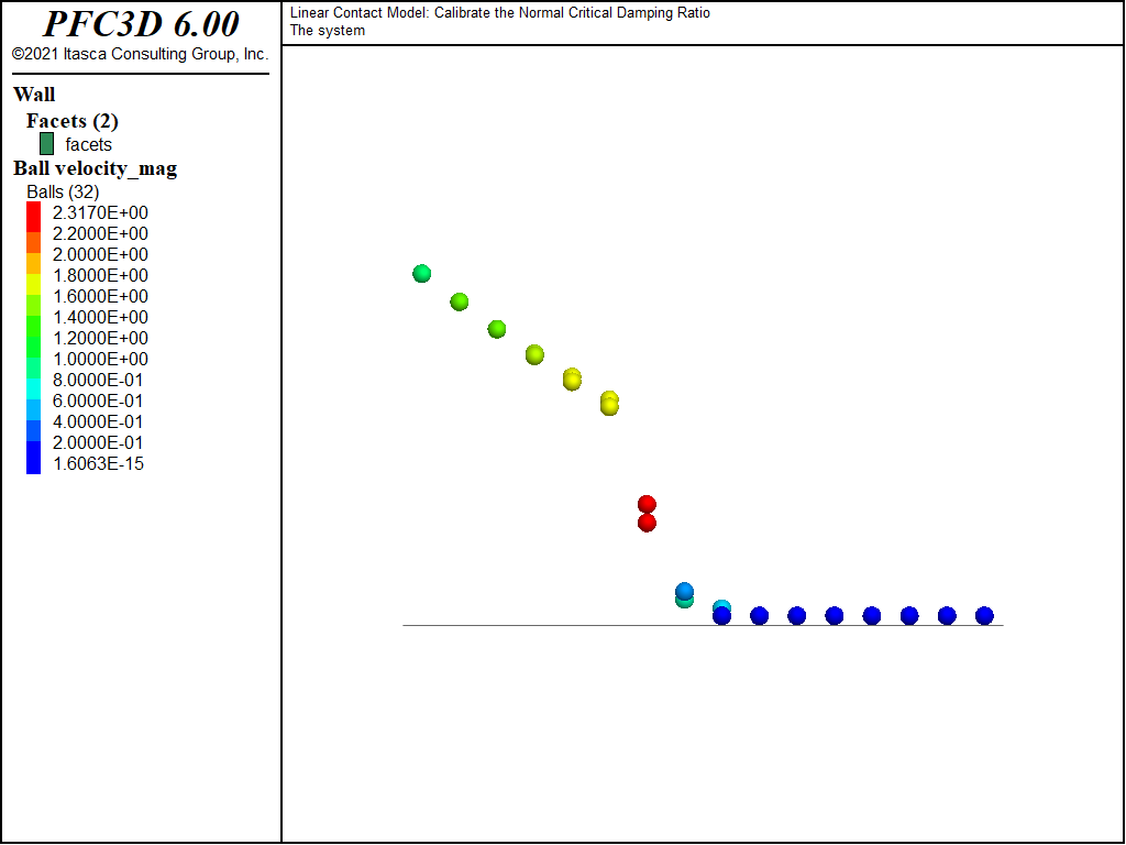
Figure 1: The system after one second of simulation.

Figures 2 and 3 show the z-position of the balls monitored during the simulation for \(M_d\) = 0 and \(M_d\) = 1, respectively, and illustrate the change in rebound height and frequency with \(\beta_n\) and \(M_d\).

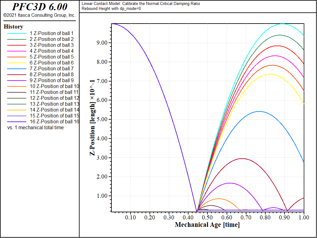
Figure 2: Ball z-position histories, \(M_d\) = 0.

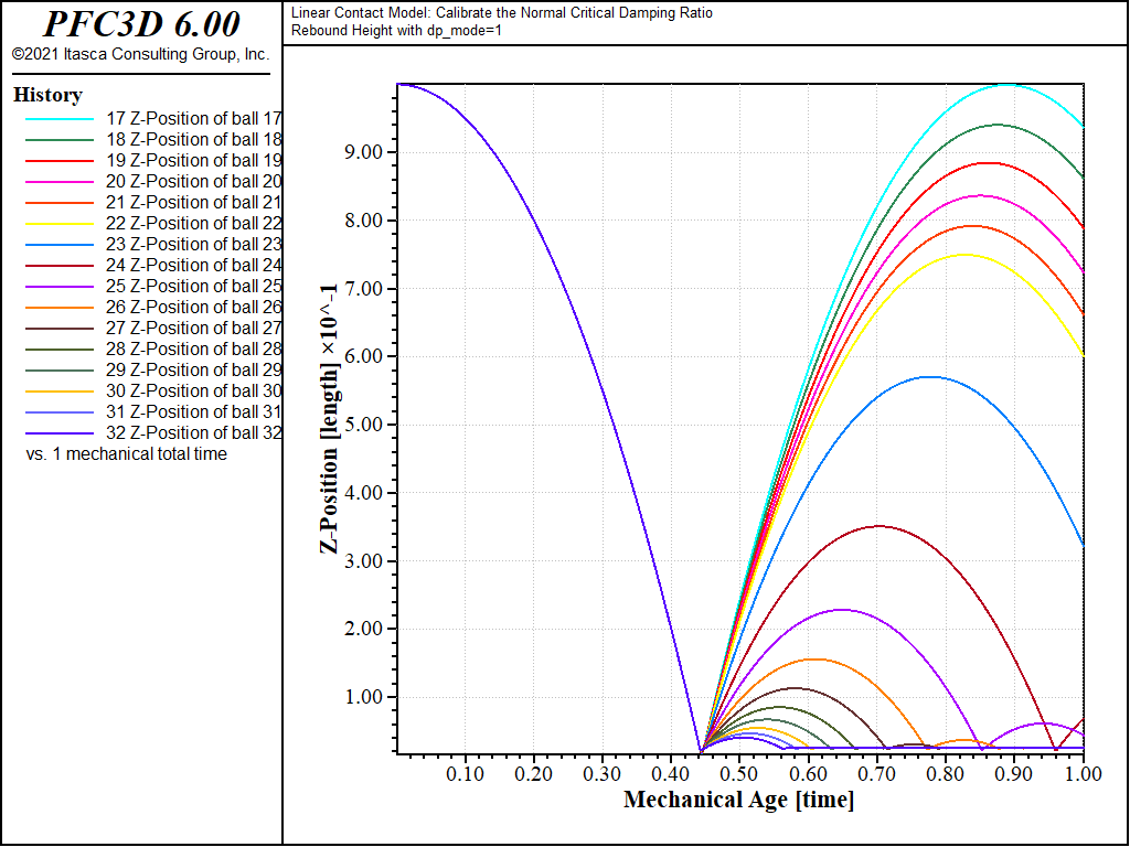
Figure 3: Ball z-position histories, \(M_d\) = 1.

The restitution coefficient is calculated from the maximum rebound height of the balls and plotted against the critical damping ratio for \(M_d\) = 0 (red marks) and \(M_d\) = 1 (green marks and dashed line) in Fig. 4, where the analytical solution given by Equation (10) is also reported (black dashed line). The maximum difference between the numerical and analytical solutions is less than 3%. Note that the accuracy of the numerical model depends on the time-integration granularity, both because the contact model implementation does and because the method chosen to evaluate the restitution coefficient in this example (measuring the rebound height) does. The results presented above are obtained with the timestep automatically evaluated by PFC. The simulation is repeated with a timestep fixed to a lower value (1 × 10^-5): the results (shown in Fig. 5) compare even better with the analytical solution (with a maximum difference less than 1%).

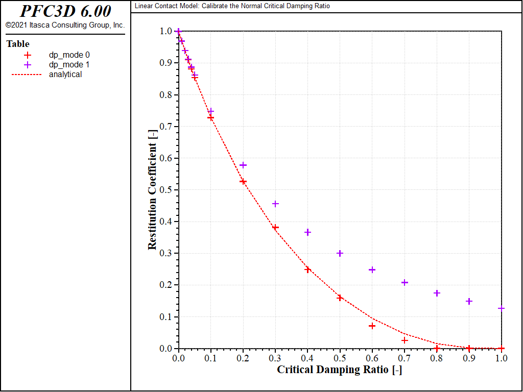
Figure 4: Relation between restitution coefficient and critical damping ratio.

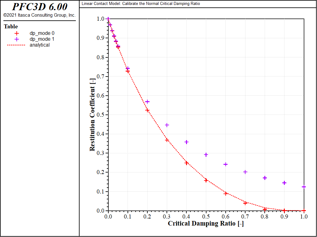
Figure 5: Relation between restitution coefficient and critical damping ratio. Simulation timestep fixed to 1 × 10^-5.

References

[Kawaguchi1992]

Kawaguchi, T. “Numerical Simulation of Fluidized Bed Using the Discrete Element Method (the Case of Spouting Bed),” in JSME (B), Vol. 58, No. 551, pp. 79-85 (1992).

Endnote

[1]

This file may be found in PFC3D under the “verification_problems/contactmodels/linear/restitution” folder in the Examples dialog (Help —> Examples on the menu). If this entry does not appear, please copy the application data to a new directory. (Use the menu commands Tools —> Copy App Data …. See the “Copy Application Data” section for details.)