Discrete Fracture Network (Advanced)

Description

Note

To view this project in 3DEC, use the menu command Help ► Examples…. Choose “3DEC/ ExampleApplications/ DFN_Advanced” and select “dfn_advanced.prj” to load. The main data files used are shown at the end of this example. All data files are found in the project.

In this example, a DFN model is defined, generated, and illustrated. A DFN model is a set of statistical distributions defining the DFN geometrical characteristics: fracture sizes, orientations, and positions. Combined with a density term and a random seed, it is used to generate DFN realizations. A DFN realization is a fracture set whose characteristics obey the statistical description of the DFN model. In this example, a DFN realization is generated from a generic DFN model. First of all, the DFN modeling framework is briefly recalled. Then, the parameters of the reference DFN model are defined and a realization is generated. The resulting DFN characteristics, including connectivity, are computed and displayed. This DFN is also used to define a simplified DFN, one that is modified to decrease numerical issues that may be encountered upon further mechanical modeling. The DFN model is defined from a classical description of fracturing (i.e., several fracture families whose respective densities are defined from apparent fracture intensity along borehole(s) and scanline(s), from bulk density or from bulk number of fractures). Thus the DFN density is calibrated to these 1D-observed fracture intensities or 3D-expected fracture densities.

Building Realizations of an Example DFN Model

The desired DFN model should have the following characteristics:

• Fractures are modeled with disks in 3D.
• Fracture orientations arise from the combination of three sets: subhorizontal, subvertical, and one more distributed (called “background fractures”).
• The background set is associated with the range of small fractures and follows a size distribution that is different from the other fracture sets with larger sizes.
• Fracture positions are uniform through space (i.e., Poisson distribution model).
• Each fracture set has a specified density.

Let us recall that fracture size, orientation, and position distributions are defined via the fracture template create command. A DFN template is a statistical description of a DFN, not an actual realization of fractures. To generate fractures consistent with the desired model, three DFN templates are necessary. Once a DFN template is defined, the corresponding fracture set density is assigned at the DFN generation stage (e.g., with the fracture generate command). A DFN realization is created with the combination of a DFN template, a density term, and a random seed. The three DFN templates are assigned power-law distributions for fracture sizes, and orientations and densities that may be derived from field observations. The subvertical and subhorizontal fracture size scaling exponent is set to 4, while the size distribution lower boundary \(l_{min}\) is equal to 10 m. Each has one preferential orientation with a given variability that is modeled by a Fisher distribution with a \(\kappa\) parameter equal to 200 for subvertical fractures and \(\kappa\) =500 for subhorizontal fractures. The Fisher distribution is a 3D symmetric analogue of the normal distribution, and is usually used to model preferential orientations with a given dispersion around the mean value (see, e.g., ([Fisher1993]).

The background fractures size scaling exponent is set to 3.2, with fracture sizes in the range [2; 10]. They have orientations bootstrapped from a user-defined distribution defined in an orientation file (see Table 1). The user-defined distribution file is basically a list of discrete values of fracture pole orientations (dip and dip direction). The statistical weight of each discrete pole orientation in the whole distribution can be increased by a multiplicative factor defined in the column Weight. This weight is commonly used to introduce an ad-hoc quantity and/or the correction (known as the Terzaghi correction) used to compensate possible orientation bias due to sampling of a 3D DFN along a 1D borehole or scanline. The Weight column is not mandatory in this user-defined distribution file. The distribution file format is the following:

• One header line.
• x lines defining the discrete distribution. Each contains an ID, followed by the 2 values of the distribution (dip and dip direction). A last (optional) column defines the quantity for these values. If not given, all values have the same probability. Separators can be a space, tab, comma, or semi-columns.
• The end of the file is specified by any empty line.

Table 1: Example of a User-Defined Orientation Distribution File

;ID	Dip	DipDirection	Weight
1	44.533	195.30	1.52
2	55.795	218.98	2.49
3	56.963	209.31	2.34
4	40.202	344.11	1.61
5	18.688	98.29	1.00
6	77.365	295.80	5.76
…

During generation, the fracture orientations are randomly selected while respecting the relative proportions of the weight column.

The densities of these sets are defined in three distinct manners. They correspond to conditions that may occur in common field cases. For the subvertical fractures, a mass density (P32) is directly provided. For the subhorizontal fractures, the density is defined so that the number of fractures (of this set) observed on a vertical outcrop section reaches a specified value. For the background fractures, the density is defined by a given P10 along a borehole (approximated by a 1D straight line). The DFN template parameters for the three fracture sets are defined in Table 2. Fracture positions are generated in a domain larger than the observation domain in order to reduce the finite-size effects. Indeed, large fractures can be observed in a given domain while their center is located outside of it. Therefore, the generation domain is increased by the largest fracture size compared to the observation domain.

Table 2: DFN Template and Density Parameters Generating the Three Fracture Sets

	Property	Distribution	Parameters
Set 1: subvertical	positions	uniform	generated in all of space
	orientations	Fisher	dip 90°, dip dir. 120°, \(\kappa\)=200
	lengths	power-law	scaling exponent \(a=4\), \(l_{min}=10\), \(l_{max}=500\)
	density		\(P_{32}\)=0.33 in the model domain extent
Set 2: subhorizontal	positions	uniform	generated in all of space
	orientations	Fisher	dip 20°, dip dir. 30°, \(\kappa\)=200
	lengths	power-law	scaling exponent \(a=4\), \(l_{min}=10\), \(l_{max}=500\)
	density		number of observed fractures on the vertical outcrop: 39
Set 3: background	positions	uniform	generated in all of space
	orientations	bootstrapped	from file
	lengths	power-law	scaling exponent \(a=3.2\), \(l_{min}=2\), \(l_{max}=10\)
	density		\(P_{10}=0.5\) measured on the vertical borehole ( \(l=85\) m)

Initialization

Prior to fracture generation, a domain must be specified via the model domain extent command. Fractures can only exist in this cubical volume and are truncated at its edges. It is possible to define (in the generation command) a generation volume and a tolerance volume with the limit that the tolerance volume is included within the domain extent. In this case, fracture positions are generated within the generation volume, but only fractures inside (either partially or completely) the tolerance volume are kept and truncated at its edges. Additionally, the initial random seed for generation is fixed so that the resulting realizations are reproducible:

model new

; define the domain
model domain extent -50 50 -50 50 -50 50

; fix the random seed
model random 101

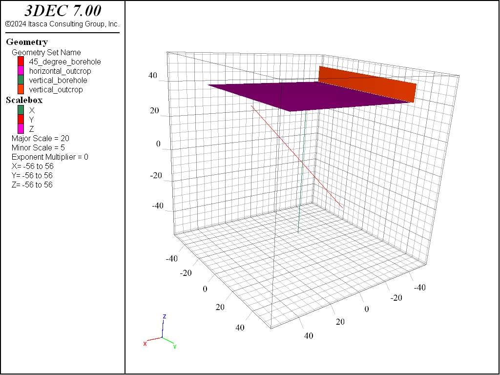
For visualization and calibration purposes, several geometry objects are defined to mimic outcrops and boreholes. It is possible to compute the intersections between fractures and 1D or 2D geometries, and analyze/visualize these intersections. Two boreholes (one vertical and one dipping 45°) plus two outcrops are defined. Outcrops are composed of a single planar (2D) polygon; boreholes are defined as 1D lines. Note that it is also possible to model boreholes by cylindrical geometries:

; borehole creations 
geom set 'vertical_borehole'
geom edge create by-position (0,0,-45) (0,0,40)

geom set '45_degree_borehole'
fish def make_45_borehole
   local x1 = -50
   local x2 = 50
   ; rotation of 45 degree
   local x1rot = x1*math.cos(math.pi/4)
   local z1rot = x1*math.sin(math.pi/4)
   local x2rot = x2*math.cos(math.pi/4)
   local z2rot = x2*math.sin(math.pi/4)
   command 
       geom edge create by-position [(x1rot,0,z1rot)] [(x2rot,0,z2rot)]
   endcommand
end
[make_45_borehole]

; outcrop creation 
geom set 'horizontal_outcrop'
geom polygon create by-position (-40,-40,40) (-40,40,40) ...
                                (40,40,40) (40,-40,40)
geom set 'vertical_outcrop'
geom polygon create by-position (-41,-41,50) (-41,41,50) ...
                                (-41,41,40) (-41,-41,40)

The geometries are illustrated by Figure 1.

Figure 1: Domain, boreholes, and outcrops.

Generation of the DFN

The three fracture sets are defined separately via DFN templates and generated in separate steps. For each set, the DFN template parameters are defined using the fracture template create command that defines the size and orientation distributions. Fractures are then generated using the fracture generate command that specifies the target density, in addition to the DFN template to be used. The generation domain is defined in the fracture generate command, while the tolerance domain is not specified because the model domain is used. For the subvertical fractures, built-in distributions are used and the two commands are rather simple. The target density, defined with the mass-density keyword, is a mass density (\(P_{32}\)) of 0.33:

; define the template of set 1: vertical fractures
fracture template create 'sub_vertical' orientation fisher 90,120,200 ...
     size power-law 4 size-limit 10 500
fracture generate dfn 'sub_vertical' generation-box ...
     -100 100 -100 100 -100 100 template 'sub_vertical' mass-density 0.33

For the subhorizontal fractures, the target density is reached when the number of fractures visible on the vertical outcrop is as specified above. Since it is not a built-in option of the generation command, we use the definition of a user-defined stopping criterion. To achieve this density, we use two FISH functions: one as a modification function (the intrinsic hori_study with the modify keyword) and one as a user-defined stopping function (the hori_stop intrinsic with the fish-stop keyword) in the fracture generate command. The modification function is called as each fracture is generated and provides, as an argument, a pointer to the fracture. In this case it is used to count the number of fractures intersecting the vertical outcrop (with the FISH intrinsics fracture.gintersect). The stopping function is called after the generation of each fracture, and the generation is stopped if the function returns 1. In this case, it is used to check if the number of fractures intersecting the vertical outcrop is the target number:

; define the template of set 2: horizontal fractures
fracture template create 'sub_horizontal' orientation fisher 20 30 500 ...
     size power-law 4 size-limit 10 500

fish define variables
  global nb_hori = 0
  global nb_hori_aimed = 39
end
[variables]

fish define hori_study(frac)
  local outc = geom.set.find('vertical_outcrop')
  local is_inter = fracture.gintersect(frac,outc)
  if is_inter>0
    nb_hori = nb_hori+1
  endif
end

fish define hori_stop
    hori_stop = 0
    if nb_hori >= nb_hori_aimed
        hori_stop=1
    endif
end

fracture generate dfn 'sub_horizontal' generation-box ...
     -100 100 -100 100 -100 100 template 'sub_horizontal' ...
     modify hori_study fish-stop hori_stop

For the third background fracture set, the density is defined by \(P_{10}\) along the vertical borehole. The borehole is specified via a geometry set with the p10 and geometry keywords to the fracture generate. Fractures are generated until the target fracture frequency or \(P_{10}\) value is reached on the borehole defined in the generation command. Note that even if the \(P_{10}\) is computed, borehole intercepts are not actually computed. In addition, one can specify the line of a borehole directly without the use of a geometry set:

; define the template of set 3: background jointing
fracture template create 'background' orientation bootstrapped ...
     'orientation_distribution.inp' size power-law 3.2 size-limit 2 10
fracture generate dfn 'background' generation-box ...
     -55 55 -55 55 -55 55 template 'background' p10 0.5 ...
     geometry 'vertical_borehole'

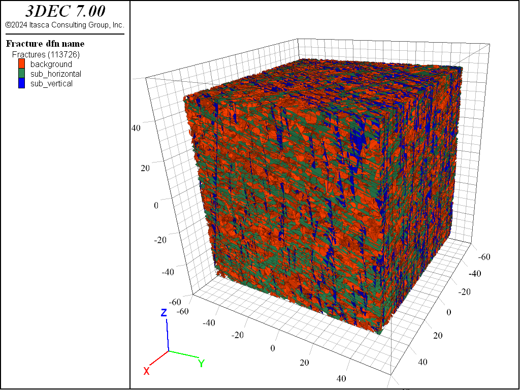
The resulting DFN (illustrated in Figure 2) contains about 110,000 fractures. This plot is obtained by adding the Fracture plot item, colored by DFN name (in Labels). The associated stereonet is illustrated in Figure 3, where the two dominant orientations are clearly visible. This plot is obtained by adding the plot item Fracture stereonet.

Figure 2: The generated DFN with the three fracture sets.

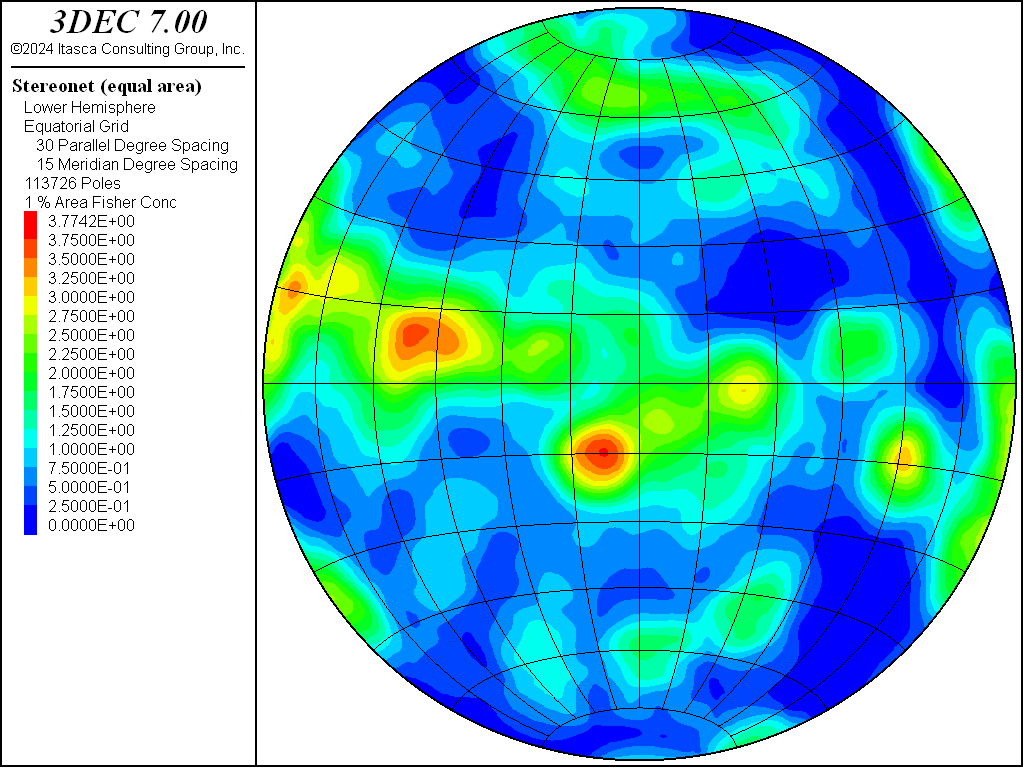
Figure 3: Stereonet of the complete DFN (equal area projection, Fisher concentrations): contour plot (1% circle area).

Analysis of the DFN

In this section, some characteristics of the DFN are analyzed. First, global DFN statistics are printed. Simple outcrop and borehole samplings are performed. The DFN connectivity is also analyzed. The analyses provided in this section are rudimentary and should be used as starting points for more advanced analyses. The fracture compute command displays the DFN density. Various densities can be output: the mass density with the mass-density keyword, the \(P_{10}\) along any line with the p10 keyword, etc. FISH intrinsics can also be used to print additional global statistics. In this case, the total fracture density (\(P_{32}\)) is equal to 1.6 m²/m³. Note that the fracture compute p10 command and the fracture.geomp21 FISH intrinsic provide fast access to DFN densities, but do not actually compute intersections. In addition, the fracture compute p10 command does not require a preexisting geometry object since it is temporarily defined in the command line.

fracture compute mass-density
fracture compute p10 begin (-50,0,0) end (50,0,0)
fish define geometry_density
    local poutcrop = geom.set.find('vertical_outcrop')
    local pborehole = geom.set.find('vertical_borehole')
    local oo = io.out('p21 vertical = '+string(fracture.geomp21(poutcrop)))
    oo = io.out('p10 vertical = '+string(fracture.geomp10(pborehole)))
end
[geometry_density]

To generate trace maps and get the intercepts along a borehole, one must first calculate the intersections between the DFN and the outcrops. Intersections between fractures and plane are called traces; intersections between fractures and lines are called intercepts. With the fracture intersections compute command and the with-geometry keyword, intersections between fractures and geometries are computed and saved in different intersection sets. Then, in order to facilitate further analysis, fracture extras are assigned an index defining whether or not they intersect one of the current geometry sets with the assign_extras FISH function. We assign the values 1, 2, and 3 to extras 1, 2, and 3, in order to identify which fractures are associated with the corresponding intersection sets. The use of various extras is explained by the fact that a fracture can simultaneously intersect several different geometries. Similar FISH functions could also be used to export trace properties.

; traces and intercepts
fracture intersection compute with-geometry 'horizontal_outcrop' ...
     intersection-set 'inter_hori_out' group-slot '1'
fracture intersection compute with-geometry 'vertical_outcrop' ...
     intersection-set 'inter_vert_out' group-slot '2'
fracture intersection compute with-geometry 'vertical_borehole' ...
     intersection-set 'inter_vert_bore' group-slot '3'

fish define assign_extras
    local set1 = fracture.inter.set.find(1)
    local intlist = fracture.inter.set.interlist(set1)
    loop foreach e1 intlist
        local f1 = fracture.inter.end1(e1)
        if type.pointer.id(f1) = fracture.typeid then
            fracture.extra(f1,1) = 1
        endif
    endloop    
    local set2 = fracture.inter.set.find(2)
    intlist = fracture.inter.set.interlist(set2)
    loop foreach e1 intlist
        f1 = fracture.inter.end1(e1)
        if type.pointer.id(f1) = fracture.typeid then
            fracture.extra(f1,2) = 2
        endif
    endloop
    local set3 = fracture.inter.set.find(3)
    intlist = fracture.inter.set.interlist(set3)
    loop foreach e1 intlist
        f1 = fracture.inter.end1(e1)
        if type.pointer.id(f1) = fracture.typeid then
            fracture.extra(f1,3) = 3
        endif
    endloop
end 

[assign_extras]

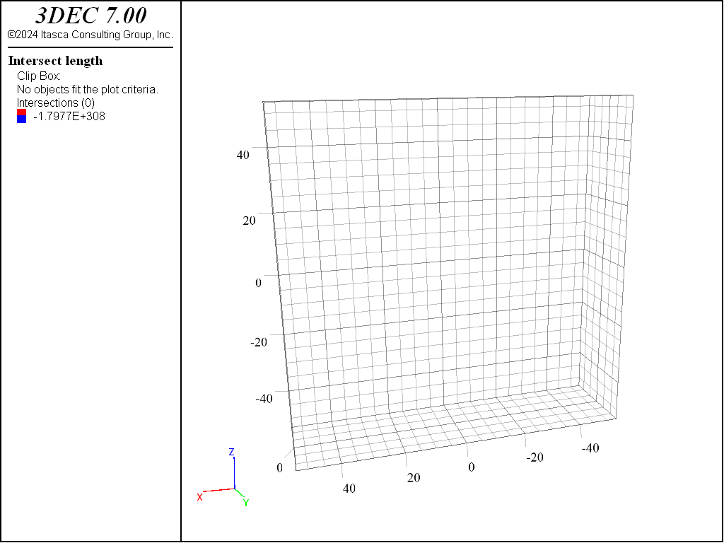
Figure 4 and Figure 5 show the two outcrop trace maps calculated with the previous code. These figures are obtained by adding the plot item DFN intersections colored by length (in Values) and by selecting, in the Display options, only the appropriate intersection set (named here inter_hori_out and inter_vert_out). In Figure 6, the fractures intersecting the vertical borehole are displayed. This is obtained by adding the plot item DFN values colored by area with a filter based on extra 3.

Figure 4: Traces on the horizontal outcrop, colored by length.

Figure 5: Traces on the vertical outcrop, colored by length.

Figure 6: Fractures intersecting the vertical borehole.

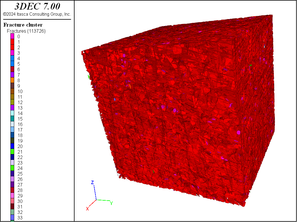
Finally, the connectivity between fractures of the DFN is analyzed. The first step is to compute intersections between fractures. The command fracture intersections compute is used again (the with-geometry keyword is not used), and yields about 500,000 intersections between fractures. The second step is to compute the clusters of connected fractures. A fracture cluster is defined as the set of intersecting fractures. In other words, there is always a connected path between any two fractures of a cluster. Conversely, two fractures in two separate clusters are disconnected. The clusters are computed with the fracture cluster command. The resulting intersections and clusters are shown by Figure 7 and Figure 8. Figure 7 is obtained by adding the plot item DFN intersections colored by length (in Values) and by selecting, in the Display options, only the set named all. Figure 8 is obtained by adding the plot item DFN values, colored by cluster (in Values). As this plot is showing, in the present case, the fractures are well-connected, with a marginal number of fractures not falling within the global cluster. However, in less connected DFNs, the organization between clusters can be much more complex:

fracture intersection compute intersection-set 'all'
fracture cluster group-slot '1' intersection-set 'all'

Figure 7: Intersections in the system colored by length.

Figure 8: Fractures colored by cluster index (blue: main cluster, green: others).

Simplification of the DFN

In some cases, a DFN may consist of so many fractures that it cannot be used in further mechanical modeling. Thus, one might need to reduce the DFN to a simplified version that captures many of the characteristics of the original DFN. In this example, we proceed with several assumptions and consecutive actions on the DFN:

• Some fractures are negligible with regard to the application and can therefore be removed:
• if they do not belong to the largest cluster of connected fractures, or
• if they are far from a given injection point.
• Fractures can be combined along common planes or merged based on proximity.

These assumptions could represent a simplification in the context of hydraulic fracture stimulations from a given point. The relevancy of the simplification assumptions are the responsibility of the user and are obviously related to specific conditions of the target application. In particular, the fracture combination (through command fracture combine) does not guarantee that all DFN characteristics are maintained. It is the user’s responsibility to assess the DFN validity for their specific purpose. First, all fractures not belonging to the largest cluster are identified. Indeed, it is assumed that only the largest cluster is connected to the reference borehole. Therefore, isolated fractures that do not belong to this cluster are deleted by using the fracture delete command with the appropriate range. Indeed, during the computation of clusters, groups are associated with clusters based on the underlying intersection set name and the cluster index (fractures in the largest cluster are grouped, in this case, in the all1 group). In practice, it is recommended that intersections and clusters be cleaned (fracture intersections delete command) before acting on the DFN in order to increase the computation speed. Intersections are computed again afterwards. Under the present conditions, most of the fractures are connected to the largest cluster and the proportion of isolated fractures is small. This simplification prunes 2000 fractures from the DFN.

; keep only infinite cluster
fracture intersection delete
fracture delete range group "all1" not
fracture intersection compute intersection-set 'all'

In the next step, fractures with too long of a “connected distance” to a defined injection section are deleted. The “connected distance” between a fracture and a reference zone (like the injection section) is the total length of the shortest connected path between the fracture and the reference (Figure 9). It is the total distance from the center of intersections between fractures that must be crossed to reach the section.

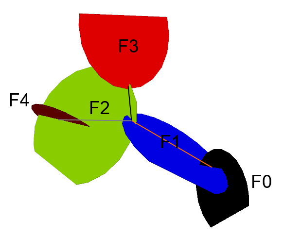
Figure 9: Illustration of the connected distance between 4 fractures and the reference illustrated by a red cube. F1 is directly connected to the reference, and the connected distance is 0. For F2, it is the size of the orange segment; for F3, it is the sum of the black segment size and the orange segment; for F4, it is the sum of the orange segment size and the grey segment size.

First, a 2D geometry defining the injection section is defined and the connected distance is computed with the fracture connectivity distance command. Next, the fractures with a “connected distance” larger than 50 m are removed. This simplification prunes an additional 75,000 fractures from the DFN. The resulting filtered DFN is shown in Figure 10 (DFN values colored by extra 6).

; filter by connected distance

geom set 'injection_section'
geom poly create by-position (-1,-1,-1) (-1,1,-1) (1,1,-1) (1,-1,-1)
geom poly create by-position (-1,-1,-1) (-1,1,-1) (-1,1,1) (-1,-1,1)
geom poly create by-position (-1,-1,1) (-1,1,1) (1,1,1) (1,-1,1)
geom poly create by-position (1,1,1) (1,-1,1) (1,-1,-1) (1,1,-1)
geom poly create by-position (1,1,1) (1,1,-1) (-1,1,-1) (-1,1,1)
geom poly create by-position (1,-1,1) (1,-1,-1) (-1,-1,-1) (-1,-1,1) 
fracture connectivity distance extra-index 6 ...
     starting-geometry 'injection_section' intersection-set '5'
fracture intersection delete
fracture delete range extra 6 0 50 not

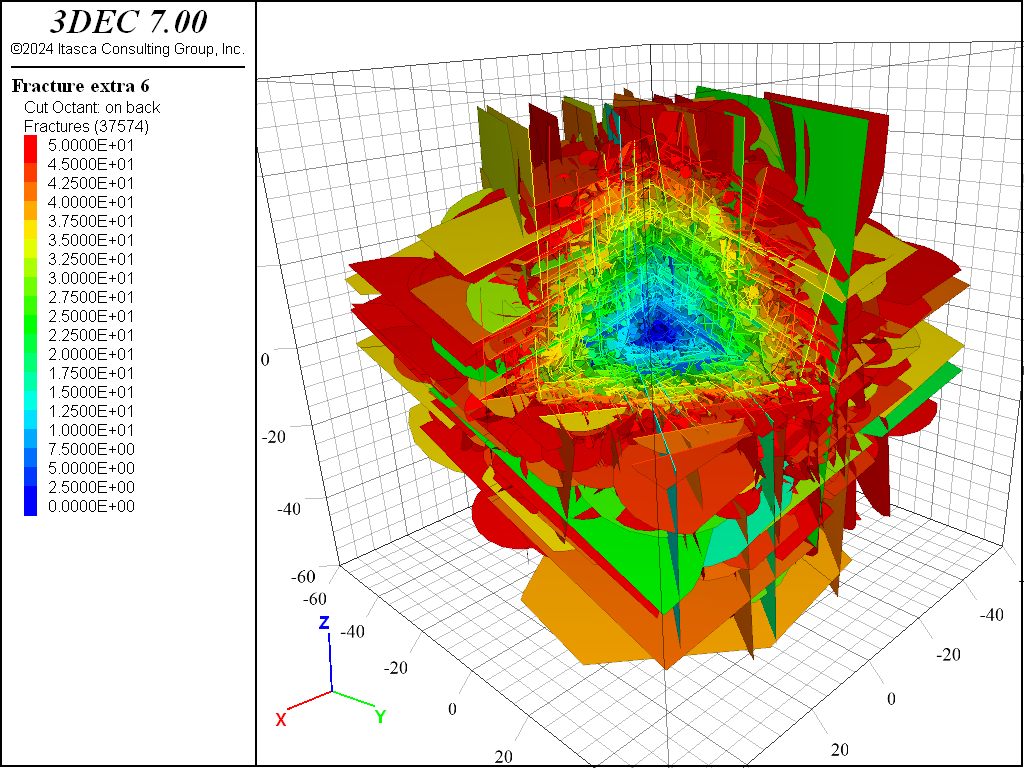
Figure 10: Simplified DFN by filtering fractures based on connectivity: only in the main cluster and with a connected distance smaller (or equal) than 50 m. Fractures are colored according to their distance to the injection section.

A further simplification is achieved by projecting fractures onto a limited number of reference planes and by combining overlapping fractures with the merge command. With this command, the plane of the largest fracture is taken as a reference. Then, smaller fractures are projected to the plane if:

• the distance between their center and the plane is smaller than a given distance; and
• if the difference between the plane orientation and the fracture orientation is smaller than a given angle.

This procedure is iterated moving from the largest fracture to the smallest one. After the projection, several fractures are coplanar and might overlap. By using the keyword merge, overlapping fractures are merged. If a fracture is completely included within a larger one, it is removed. The combination is made with three sets of criteria, depending on the distance between fractures and the injection point. This could reflect conditions where the influence of fractures on the results is strong close to the injection, while the influence of the furthest fractures is less important. The closest fractures are merged based on strict criteria, while the furthest fractures are merged using less strict criteria. An additional 33,000 fractures are pruned from the DFN with this step.

; fracture combination


fracture combine distance 1 angle 20 merge range extra 6 10 20 
fracture combine distance 5 angle 45 merge range extra 6 20 30 
fracture combine distance 10 angle 80 merge range extra 6 30 50 

The resulting DFN has approximately 4,000 fractures and is shown in Figure 11 (DFN values colored by extra 6).

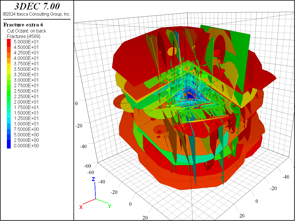
Figure 11: Simplified DFN by projection in reference planes and combination of overlapping fractures.

Creating the 3DEC model

We can now create a 3DEC model from the DFN. Add a new data file to the project and enter the following commands to create 100 × 100 × 100 m block, and divide it into 64 smaller blocks:

model restore 'simplification2'
block create brick -50 50 -50 50 -50 50
block densify segments 4 4 4 joint-set 99

A joint-set ID of 99 is assigned to these joints since they are fictitious and you probably want to be able to identify them and give them different properties from the actual joints created with the DFN. The DFN is simulated in 3DEC in the following way:

1. Fractures are sorted from largest to smallest.
2. Starting with the largest fracture, all blocks not touching the fracture are hidden.
3. Visible blocks are cut.
4. All blocks are shown again.
5. Repeat steps 2 to 5 with increasingly smaller fractures.

This process explains why it is advisable to densify the initial large block. This will prevent the first few fractures from forming very long cuts, since the densification will allow some blocks to be hidden.

The procedure described above is performed with a single command for each DFN. In this example we will only make cuts corresponding to the subhorizontal and subvertical fracture sets. The background fractures are still too dense for 3DEC to be able to create usable convex blocks. The background fractures can be simplified further if required, or they could be accounted for by lowering the stiffness and strength of the blocks according to some classification scheme (e.g., Geological Strength Index).

Before the cuts are made it is a good idea to set the tolerance to a low value since there are many fractures, and the default tolerance will result in cuts being rejected due to the formation of small blocks. Add the following commands to your data file:

block tolerance 0.001
block cut dfn name 'sub_vertical'
block cut dfn name 'sub_horizontal'

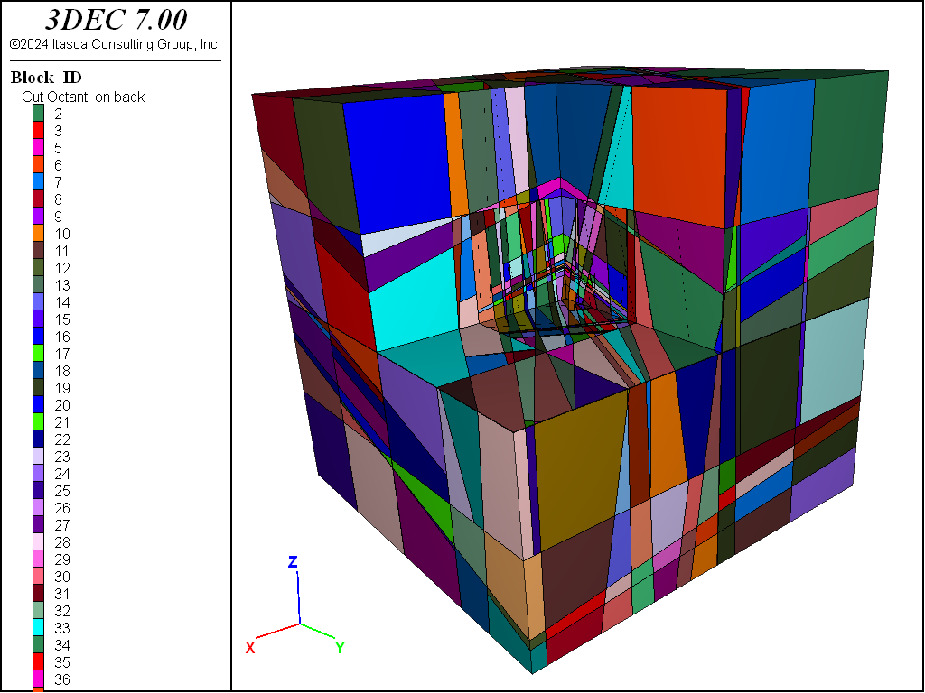
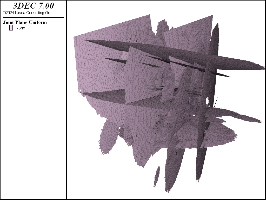
Add a plot of blocks. Add an octant cutting plane and plot the blocks behind the octant. The plot should appear as in Figure 12.

Figure 12: Blocks after densification and cutting with the horizontal and vertical fracture sets.

The fractures in the DFN are circular and finite in extent. However in 3DEC, blocks cannot be partially cut, so all of the 3DEC joints are necessarily bigger than the corresponding fractures in the DFN. We can account for this by assigning different joint properties to areas lying inside of the circular fractures and areas outside of the circular fractures. This idea is illustrated in Figure 13.

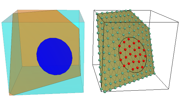
Figure 13: Illustration of how sub-contacts on a joint plane can be assigned different properties inside (red) and outside (light blue) of a circular fracture

To do this, we first need to zone the blocks. An edge length of 2 is sufficient for this example. Then contact constitutive models and properties are then assigned. First the construction joints are set to be elastic and a normal and shear stiffness are assigned. Then the DFN joints are given a Mohr-Coulomb constitutive model. All of the DFN fractures are assigned a high cohesion and tension, but then the subcontacts inside of the fractures are assigned 0 cohesion and tension by using the range :kwd:`dfn-3dec’. The commands are shown below.

; construction joints
block contact jmodel assign elastic range joint-set 99
block contact property stiffness-normal 1e10 stiffness-shear 1e10 ...
  range joint-set 99

; DFN fractures
block contact jmodel assign mohr range joint-set 99 not

; outside properties
block contact property stiffness-normal 1e10 stiffness-shear 1e10 friction 20 ...
  cohesion 1e6 tension 1e6 range joint-set 99 not

; inside properties
block contact property stiffness-normal 1e10 stiffness-shear 1e10 friction 20 ...
  cohesion 0 tension 0 range dfn-3dec 'sub_vertical' 'sub_horizontal'

model save 'dfn_3dec'

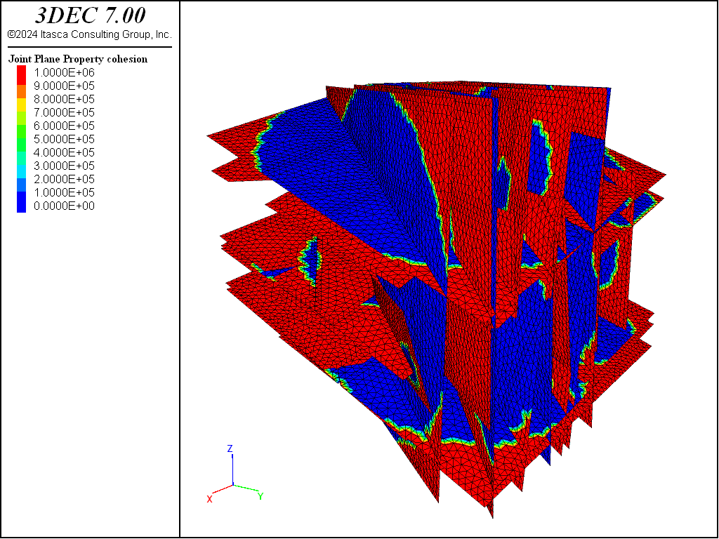
The DFN in 3DEC can be visualized by plotting joint contours of property (Figure 14). Choose cohesion for the property being plotted. You can then hide the fictitious joints created by the BLOCK DENSIFY command by clicking the range icon next to the plot item, selecting Joint ID from the range list, checking the Not box and entering 99 for the ID. You can now see circular section of faults with dark colors corresponding to 0 cohesion, and other sections of faults with very high cohesion.

Figure 14: Joints created by cutting with the DFN contoured according to cohesion.

An easy way to plot only the portions of the joints inside of the DFN fractures is to use the DFN Distance range item in the plot. Figure 15 shows the result of plotting the joints within a distance of 0.01 from the sub_vertical and sub_horizontal DFNs.

References

[Fisher1993]

Fisher, N. I. Statistical Analysis of Circular Data. Cambridge University Press (1993).

Data Files

dfn_create.dat

;-----------
;  CODE 1
;-----------

; excerpt-init-start
model new

; define the domain
model domain extent -50 50 -50 50 -50 50

; fix the random seed
model random 101
; excerpt-init-end

;-----------
;  CODE 2
;----------- 

; excerpt-bhss-start
; borehole creations 
geom set 'vertical_borehole'
geom edge create by-position (0,0,-45) (0,0,40)

geom set '45_degree_borehole'
fish def make_45_borehole
   local x1 = -50
   local x2 = 50
   ; rotation of 45 degree
   local x1rot = x1*math.cos(math.pi/4)
   local z1rot = x1*math.sin(math.pi/4)
   local x2rot = x2*math.cos(math.pi/4)
   local z2rot = x2*math.sin(math.pi/4)
   command 
       geom edge create by-position [(x1rot,0,z1rot)] [(x2rot,0,z2rot)]
   endcommand
end
[make_45_borehole]

; outcrop creation 
geom set 'horizontal_outcrop'
geom polygon create by-position (-40,-40,40) (-40,40,40) ...
                                (40,40,40) (40,-40,40)
geom set 'vertical_outcrop'
geom polygon create by-position (-41,-41,50) (-41,41,50) ...
                                (-41,41,40) (-41,-41,40)
; excerpt-bhss-end
model save 'geometries'


;------------
;  CODE 3
;------------

; excerpt-gnfs-start
; define the template of set 1: vertical fractures
fracture template create 'sub_vertical' orientation fisher 90,120,200 ...
     size power-law 4 size-limit 10 500
fracture generate dfn 'sub_vertical' generation-box ...
     -100 100 -100 100 -100 100 template 'sub_vertical' mass-density 0.33
; excerpt-gnfs-end

;-----------
;  CODE 4
;-----------

; excerpt-set2-start
; define the template of set 2: horizontal fractures
fracture template create 'sub_horizontal' orientation fisher 20 30 500 ...
     size power-law 4 size-limit 10 500

fish define variables
  global nb_hori = 0
  global nb_hori_aimed = 39
end
[variables]

fish define hori_study(frac)
  local outc = geom.set.find('vertical_outcrop')
  local is_inter = fracture.gintersect(frac,outc)
  if is_inter>0
    nb_hori = nb_hori+1
  endif
end

fish define hori_stop
    hori_stop = 0
    if nb_hori >= nb_hori_aimed
        hori_stop=1
    endif
end

fracture generate dfn 'sub_horizontal' generation-box ...
     -100 100 -100 100 -100 100 template 'sub_horizontal' ...
     modify hori_study fish-stop hori_stop
; excerpt-set2-end

;-----------
;  CODE 5
;-----------

; excerpt-set3-start
; define the template of set 3: background jointing
fracture template create 'background' orientation bootstrapped ...
     'orientation_distribution.inp' size power-law 3.2 size-limit 2 10
fracture generate dfn 'background' generation-box ...
     -55 55 -55 55 -55 55 template 'background' p10 0.5 ...
     geometry 'vertical_borehole'
; excerpt-set3-end


model save 'dfngeneration'

;-----------
;  CODE 6
;-----------

; print densities

; excerpt-dens-start
fracture compute mass-density
fracture compute p10 begin (-50,0,0) end (50,0,0)
fish define geometry_density
    local poutcrop = geom.set.find('vertical_outcrop')
    local pborehole = geom.set.find('vertical_borehole')
    local oo = io.out('p21 vertical = '+string(fracture.geomp21(poutcrop)))
    oo = io.out('p10 vertical = '+string(fracture.geomp10(pborehole)))
end
[geometry_density]
; excerpt-dens-end

;-----------
;  CODE 7
;-----------

; excerpt-tnis-start
; traces and intercepts
fracture intersection compute with-geometry 'horizontal_outcrop' ...
     intersection-set 'inter_hori_out' group-slot '1'
fracture intersection compute with-geometry 'vertical_outcrop' ...
     intersection-set 'inter_vert_out' group-slot '2'
fracture intersection compute with-geometry 'vertical_borehole' ...
     intersection-set 'inter_vert_bore' group-slot '3'

fish define assign_extras
    local set1 = fracture.inter.set.find(1)
    local intlist = fracture.inter.set.interlist(set1)
    loop foreach e1 intlist
        local f1 = fracture.inter.end1(e1)
        if type.pointer.id(f1) = fracture.typeid then
            fracture.extra(f1,1) = 1
        endif
    endloop    
    local set2 = fracture.inter.set.find(2)
    intlist = fracture.inter.set.interlist(set2)
    loop foreach e1 intlist
        f1 = fracture.inter.end1(e1)
        if type.pointer.id(f1) = fracture.typeid then
            fracture.extra(f1,2) = 2
        endif
    endloop
    local set3 = fracture.inter.set.find(3)
    intlist = fracture.inter.set.interlist(set3)
    loop foreach e1 intlist
        f1 = fracture.inter.end1(e1)
        if type.pointer.id(f1) = fracture.typeid then
            fracture.extra(f1,3) = 3
        endif
    endloop
end 

[assign_extras]
; excerpt-tnis-end

model save 'traces'

;-----------
;  CODE 8
;-----------

; connectivity

; excerpt-kelx-start
fracture intersection compute intersection-set 'all'
fracture cluster group-slot '1' intersection-set 'all'
; excerpt-kelx-end

model save 'connectivity'

;-----------
;  CODE 9
;-----------

; excerpt-wlns-start
; keep only infinite cluster
fracture intersection delete
fracture delete range group "all1" not
fracture intersection compute intersection-set 'all'
; excerpt-wlns-end

;-----------
;  CODE 10
;-----------

; excerpt-lake-start
; filter by connected distance

geom set 'injection_section'
geom poly create by-position (-1,-1,-1) (-1,1,-1) (1,1,-1) (1,-1,-1)
geom poly create by-position (-1,-1,-1) (-1,1,-1) (-1,1,1) (-1,-1,1)
geom poly create by-position (-1,-1,1) (-1,1,1) (1,1,1) (1,-1,1)
geom poly create by-position (1,1,1) (1,-1,1) (1,-1,-1) (1,1,-1)
geom poly create by-position (1,1,1) (1,1,-1) (-1,1,-1) (-1,1,1)
geom poly create by-position (1,-1,1) (1,-1,-1) (-1,-1,-1) (-1,-1,1) 
fracture connectivity distance extra-index 6 ...
     starting-geometry 'injection_section' intersection-set '5'
fracture intersection delete
fracture delete range extra 6 0 50 not
; excerpt-lake-end

model save 'simplification1'

;-----------
;  CODE 10
;-----------

; excerpt-snel-start
; fracture combination


fracture combine distance 1 angle 20 merge range extra 6 10 20 
fracture combine distance 5 angle 45 merge range extra 6 20 30 
fracture combine distance 10 angle 80 merge range extra 6 30 50 
; excerpt-snel-end

model save 'simplification2'

dfn_3dec.dat

; excerpt-block-start
model restore 'simplification2'
block create brick -50 50 -50 50 -50 50
block densify segments 4 4 4 joint-set 99
; excerpt-block-end

; excerpt-cut-start
block tolerance 0.001
block cut dfn name 'sub_vertical'
block cut dfn name 'sub_horizontal'
; excerpt-cut-end

; excerpt-zone-start
block zone generate edgelength 2
; excerpt-zone-end

; excerpt-joints-start
; construction joints
block contact jmodel assign elastic range joint-set 99
block contact property stiffness-normal 1e10 stiffness-shear 1e10 ...
  range joint-set 99

; DFN fractures
block contact jmodel assign mohr range joint-set 99 not

; outside properties
block contact property stiffness-normal 1e10 stiffness-shear 1e10 friction 20 ...
  cohesion 1e6 tension 1e6 range joint-set 99 not

; inside properties
block contact property stiffness-normal 1e10 stiffness-shear 1e10 friction 20 ...
  cohesion 0 tension 0 range dfn-3dec 'sub_vertical' 'sub_horizontal'

model save 'dfn_3dec'
; excerpt-joints-end