
P2PSand Model*
Note
*This model is available in FLAC3D only.
P2PSand model (Cheng and Detournay, 2021) refers to a Practical TWO-surface Plastic SAND constitutive model for general 3D geotechnical earthquake engineering application aimed at capturing essential soil dynamic characteristics. The model is a modified extension of the fabric-dilatancy related sand plasticity DM04 model developed by Dafalias and Manzari (2004). By revising some formula without adding too much complexity, improved performances are achieved with matches between the simulated results and various laboratory or field observations and empirical relationships with various initial and loading conditions. The modified model switches all void-ratio related constitutive ingredients to be relative density related, and embraces an easier calibration procedure in terms of in-situ data, such as normalized blow counts instead of experimental data in the laboratory, while it preserves the very important property of the latter to use only. The model follows the general multiaxial formulation of the DM04 model, and thus can be used for general 3D boundary value problems. The model preserves the feature that one set of model constants to simulate different responses with different initial relative densities and initial stress states.
Formulations
Elastic Law
For simplicity, this model adopts the hypoelastic formula in the elasticity part as proposed in the original DM04 model. The incremental form of the elastic part is
where \(p\) is the mean pressured defined by \(p=-tr(\boldsymbol{\sigma})/3\), \(\boldsymbol{s}\) is the deviatoric stress tensor defined by \(\boldsymbol{s} = \boldsymbol{\sigma} + p\boldsymbol{I}\) with \(\boldsymbol{I}\) is the unit tensor, \(\varepsilon_v\) is the volumetric strain with the definition of \(\varepsilon_v = tr(\boldsymbol{\varepsilon})\), \(\boldsymbol{\epsilon}\) is the deviatoric strain tensor defined by \(\boldsymbol{\epsilon}=\boldsymbol{\varepsilon}-(\varepsilon_v/3)\boldsymbol{I}\), and \(K\) and \(G\) are elastic bulk and shear modulus, respectively.
The p2PSand model considers the elastic modulus as a function of the current mean pressure \(p\) and current relative density \(D_r\):
where \(v\) is the Poisson’s ratio, \(p_{atm}\) is a reference pressure (usually the atmospheric pressure), \(G_r\) is a material parameter which is supposed to be a function of \(D_r\), and the exponent \(n\) is usually in the range of [0.4, 1.0] with a default value of 0.5 for most sands. Cheng (2018) has shown that a linear function
provides high correlation for both laboratory and in-situ sands in a range of \(0.15 \le D_r \le 0.85\) corresponding to \(1 \le (N_1)_{60} \le 33\), hence practically more complex nonlinear relationships of shear modulus in terms of \(D_r\) may not be necessary, since soil with \((N_1)_{60} \lt 1\) is not suitable for almost any construction and soil with \((N_1)_{60} \gt 33\) is usually considered non-liquefiable and a simpler constitutive model can be alternatively used. Regression based on the field data (Andrus and Stokoe II 2000) supports \(G_r = 1240 (D_r + 0.01)\), which is also the default relation in the model. Nevertheless, users can still input a non-linear \(G_r\) using a FISH function.
Critical State
Following the same motivation that the relative density is more favorable to be calibrated from the in-situ data, we propose a similar power law for the critical state but defined in terms of relative density \(D_r\) rather than the void ratio \(e\):
where \(D_{rc0}\), \(\lambda_c\), and \(\xi\) are material parameters and \(\xi = 0.7\) can be used for most sands.
Alternatively, a two-parameter logarithmic form of critical state may be derived as a function of relative density, \(D_r\), as
assuming that the critical state is reached when the relative dilatancy index (Bolton 1986), \(I_R = -D_r \ln{( {p}/{p_c} )}\), is zero. For quartzic sands, the material parameters were suggested to be \(Q = 10\) and \(R = 1\).
In the implemented version of the model in FLAC3D, the user can have options to select one of the 3-parameter or 2-parameter critical states. The 3-parameter critical state relation is expected to have more flexibility to fit wider experimental data.
Lode Angle Dependency
The P2PSand model adopts the function:
to interpolate \(M_{\theta}=g(\theta,c) M_C\) for a given Lode angle \(\theta\) and the strength ratio \(c\), which is defined by \(c=M_E/M_C=(3-\sin{\phi_{cs}})/(3+\sin{\phi_{cs}})\), with \(M_E\) the triaxial compression strength, \(M_C\) the triaxial extension strength, and \(\phi_{cs}\) the friction angle at the critical state.
Bounding and dilatancy Surfaces
The P2PSand model adopts a power form of dependence of the bounding and dilatancy surfaces on \(I_p\) by:
where \(n^b\) and \(n^d\) are material constants. A typical value of \(n^b\) is \(n^b = 0.16 - \phi_{cs}/400\) with \(\phi_{cs}\) (in degrees) is the friction angle in the critical state; Typical values of \(n^d\) is \(n^d = (4 \sim 7) n^b\). For \(M^d\), the cut-off of \(M^b \geq M^c\) is in fact forbidden so that \(M^d\) can become smaller and greater than \(M^c\). A cut-off for \(M^d\) is used when the mean pressure \(p\) is small, implying that the dilatancy ratio \(M^d/M^c\) cannot be smaller than a fixed value \(K^d_{LB}\) which is an input value usually between 0.5 to 0.8.
Yield Function
The elastic domain in the stress space is a small cone and the yield surface is defined by the same function as in DM04 model:
where \(\boldsymbol{r} = \boldsymbol{s}/p\) is the deviatoric stress-ratio tensor, \(\boldsymbol{\alpha}\) is the deviatoric back stress-ratio, and \(m\) is usually a relatively small value compared with \(M^c\). In this model, we do not take \(m\) as a dependent material constant but with a fixed value of \(m = 0.01 M^c\). The gradient to the yield surface at \(\boldsymbol{m}\) is then
where
and \(\boldsymbol{n}\) satisfies \(tr(\boldsymbol{n})=0\), \(\boldsymbol{n}:\boldsymbol{n}=1\), and \(\cos{3\theta}=-\sqrt{6} \times tr(\boldsymbol{n}^3)\).
As described in the DM04 model, if one draws from origin a line parallel to \(\boldsymbol{n}\), the line will intersect the bounding and dilatancy surfaces at at image back-stress ratio tensors \(\boldsymbol{\alpha}^b_{\theta}\) and \(\boldsymbol{\alpha}^d_{\theta}\), respectively:
Plastic Shear Modulus
In the P2PSand model, the plastic shear modulus could be proposed so that
While the above equation was shown to be effective for monotonic loading, it has not overcome two shortcomings of the DM04 model during cyclic loading: one is the repeating stress-path without further increases in shear strain amplitude after some cycles; the other is the overly high damping ratio at relative large shear strain. Recalling the great advantage of bounding surface plasticity to define at will the coefficient of \(K_p\) (as long as \(K_p=0\) on the bounding surface), and in order to improve cyclic performance, two supplementary factors \(f_1\) and \(f_2\) are added into the \(K_p\) formula for the P2PSand model:
where \(f_1\) and \(f_2\) are functions introduced to improve performance. \(f_1\) is basically a degradation factor of plastic stiffness and is introduced in order to eliminate the phenomenon of repeating stress-path without further increases in shear strain amplitude. \(f_2\) is introduced in order to reduce the hysteretic loop areas (damping ratios) at a higher shear strain.
In the P2PSand model, the so-called maximum stress-ratio surface (Figure 1) will be recorded, which has the same shape as the bounding or dilatancy surface but its size is determined by the historic position of \(\boldsymbol{\alpha}\), with the maximum radius along the \(\boldsymbol{r}_1\) direction in the \(\pi\) plain to be
where \(\theta_{\alpha}\) is the Lode angle of the current back-stress ratio tensor.
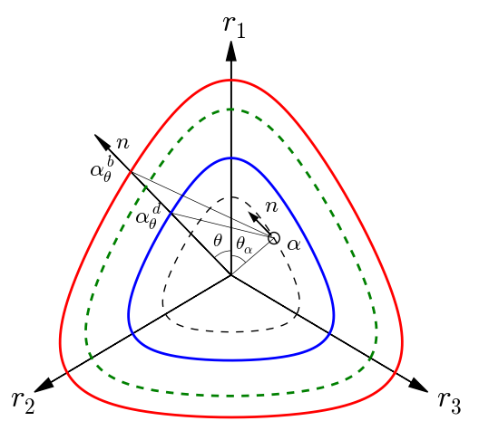
Figure 1: Schematic of surfaces in the \(\pi\) plain: bounding surface (red); dilatancy surface (blue); critical-state surface (green dash), maximum stress-ratio surface (black dash), and the yield surface (black circle).
Volumetric Plastic Strain
The increment form of the plastic volumetric strain is given by
In the P2PSand model, the dilatancy \(D\) is given by
for virginal loading (\({\parallel \boldsymbol{\alpha} \parallel}/{g(\theta_{\alpha}, c)} \geq M^m_C\)), where \(A_d\) is related to the fabric dilatancy tensor \(z\) which will be described later. When the fabric dilatancy is not significant or not developed, \(A_d=A_{d0}\), where \(A_{d0}\) is a material parameter, which can be calibrated from the monotonic triaxial compression tests.
If the state is within the maximum stress-ratio surface, the dilatancy is reduced by a factor \([K_{c} (\boldsymbol{\alpha}-\boldsymbol{\alpha}_{in}):\boldsymbol{n}]\). \(K_{c}\) is an adjusting parameter for cyclic loading or non-backbone loading path. For the virgin or backbone loading, \(K_{c}=1\). The parameter \(K_{c}\) aims at capturing the sand characteristic that the dilation/contraction evolution rate is slightly different between a virgin loading and a cyclic loading, thus pre-histories effect can be partially captureed. To match the model with the empirical CRR versus \((N_1)_{60}\) (or other measurement such as \(q_{c1N}\)) for cyclic simulations, \(K_{c}\) is suggested be calibrated last.
Fabric Evolution
Following the DM04 model, the parameter \(A_d\) is given by
where \(A_{d0}\) is a material parameter.
The increment of the fabric dilatancy tensor in the P2PSand model is
where \(c_z\) and \(z_{max}\) are material parameters. The default initialized values are \(c_z = G_r\) and \(z_{max} = \min{(21 D_r^{3.85}, 15)}\).
Elastic Modulus Degradation
In the P2PSand model, the elastic modulus is degraded during the cyclic loading to better simulate the deformation which may be underestimated otherwise. A degradation factor \(F_d\) is multiplied to the elastic moduli.
where \(k_d\) is material parameter, \(\max{\|\boldsymbol{z}}\|\) is the maximum magnitude of the fabric dilatancy tensor, and \(\int^{\boldsymbol{z}}_{\boldsymbol{0}} \|d\boldsymbol{z}\|\) is the accumulated magnitude of the the fabric dilatancy tensor, respectively. \(F_d\) remains the initial value of 1 when no fabric dilatancy develops. A low-bound value of 0.02 is set to \(F_d\). By default, \(k_d = 0.46 - 0.35D_r\) in the model but it can be overwritten by the user.
Model Parameters
The model parameters (or called properties) can be grouped into two categories: parameters for initial condition and parameters for material property.
Parameters for initial condition
The parameters for initial condition include the initial relative density and initial effective stress. These parameters for are used to initialize other parameters.
Initial Stress
Since the model is a stress-dependent constitutive model, reasonable initial stress status should be input at the first time the model is assigned. The input initial stress \(\boldsymbol{\sigma^{ini}}\) (input in terms of its six components) should be reasonable: the corresponding initial confining pressure should be positive and they should not be out-side of the bounding surface.
Before assigning this model, the zones are suggested to be initialized reasonable stresses, and/or be in mechanical equilibrium using the Mohr-Coulomb (MC) model. The MC model parameters are suggested to have zero cohesion, zero tension strength and zero dilation angle, and a friction angle with the same value as \(\phi_{cs}\). The initial stress component parameters can be input by commands, or can be input by a FISH function. Below is an example FISH function after the zone stresses have been initialized:
fish operator ini_stress(z, modelname)
    if zone.model(z) == modelname then
        local pp = zone.pp(z)
        zone.prop(z,'stress-xx-initial') = zone.stress.xx(z) + pp
        zone.prop(z,'stress-yy-initial') = zone.stress.yy(z) + pp
        zone.prop(z,'stress-zz-initial') = zone.stress.zz(z) + pp
        zone.prop(z,'stress-xy-initial') = zone.stress.xy(z)
        zone.prop(z,'stress-yz-initial') = zone.stress.yz(z)
        zone.prop(z,'stress-xz-initial') = zone.stress.xz(z)
    endif
end
[ini_stress(::zone.list, 'p2psand')]
Initial Relative Density or Normalized Blow-counts in Field Condition
The initial relative density \(D_r^{ini}\) or \((N_1)_{60}\) in field condition is an important parameter which has significant effects on the sand behaviors. The initial relative density should be input as a fraction, not in percentage. For any input value less than 0.05 the implemented version of the model in FLAC3D will reset it to 0.05; For any input value greater than 0.95 the implemented version of the model in FLAC3D will reset it to 0.95. A value less than 0.15 (corresponding to \((N_1)_{60} \leq 1\)) is not recommended. This parameter is better referred to a nominal initial relative density which approximately corresponds to the naturally deposited and normally consolidated clean sand in the field environment.
If the value of normalized blow-counts, \((N_1)_{60}\) in field condition, is available, it can be directly input as material property in place of \(D_r^{ini}\). In this model, the default correlation between \((N_1)_{60}\) and \(D_r^{ini}\) is
If the field test is the CPT data, \(D_r\) can be estimated (Mayne 2009) as
where \(q_{c1N}=(q_c/p_{atm})/(\sigma^{\prime}_{v0}/p_{atm})^{0.5}\) is the stress-normalized cone tip resistance, and \(b_x= 0.675\) for normally-consolidated (in median compressibility) clean sands such as siliceous sands (approximately equal parts of quarts and felspar); \(b_x= 0.525\) for sands with high compressibility, including mica sands, calcareous sands, and carbonate sands; \(b_x= 0.825\) for sands of low compressibility including those of quartz. Alternative estimation (Kulhawy and Mayne 1990) in terms of \(q_{c1N}\) is
where \(Q_x\) is a factor equal to 0.91, 1.0 and 1.09 for high, median and low compressibility sands, respectively. Another empirical expression (Idriss and Boulanger 2008) of \(D_r\) in term of \(q_{c1N}\) is
Parameters for material property
The parameters for material property can be further grouped into three sub-categories: primary, auxiliary and constant parameters. The primary parameters have some larger influence on the simulated response by the model. The auxiliary parameters have less influence on model responses, which usually need no further refinements. Nevertheless, reliable experimental data are needed to support the selection of appropriate values for these parameters. The only constant parameter is the reference pressure, which should be always referred to the standard atmospheric pressure for the purpose of normalization of stress or pressure.
Except for the parameters necessary for initial conditions, which require correct initialization to represent the in-situ conditions, all other model parameters have default values which have been internally calibrated for in-situ sands.
The default values of the parameters are selected to predict CRR values from the single-zone (or called single-element) direct simple shear (DSS) simulations with the following criteria:
- At an event equivalent to an earthquake with a magnitude about 7.5;
- Effective overburden pressure (\(\sigma^{\prime}_{v0}\)) is about 100 kPa (~ 1 atm);
- Lateral earthquake pressure coefficient at rest is \(K_0=0.5\);
- Target CRR values are close to the state-of-practice criteria (Figure 2), e.g., SPT clean-sand base curve from liquefaction case histories (e.g., by Youd et al, 2001);
- Arrive a S.A. (single-amplitude) peak shear strain of about 3%, or D.A. (double-amplitude) shear strain of about 6%, whichever comes first, with approximately 15 cycles.
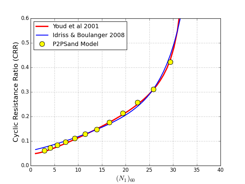
Figure 2: Values of CRR predicted by the model and compared to semi-empirical curves.
References
Andrus, R.D. and Stokoe II, K.H. “Liquefaction resistance of soils from shear-wave velocity.” Journal of Geotechnical and Geoenvironmental Engineering, 126(11), 1015–1025 (2000).
Bolton, M. “The strength and dilatancy of sands.” Geotechnique, 36(1), 65–78 (1986).
Cheng, Z. A practical 3D bounding surface plastic sand model for geotechnical earthquake engineering application. in Geotechnical Earthquake Engineering and Soil Dynamics V: Numerical Modeling and Soil Structure Interaction, ASCE, 34–37 (2008).
Cheng, Z. and Detournay D. “Formulation, validation and application of a practice-oriented two-surface plasticity sand model.” Computers and Geotechnics, 132(4), 103984 (2021). https://doi.org/10.1016/j.compgeo.2020.103984.
Dafalias, Y. F. and Manzari, M. T. “Simple plasticity sand model accounting for fabric change effects,” Journal of Engineering mechanics, 130(6), 622–634 (2004).
Idriss, I. M. and Boulanger, R. W. Soil liquefaction during earthquakes. Earthquake Engineering Research Institute (2008).
Mayne, P. Engineering design using the cone penetration test: geotechnical applications guide. ConeTec Investigation Inc (2009).
Youd, T., et al. “Liquefaction resistance of soils: Summary report from the 1996 NCEER and 1998 NCEER/NSF workshops on evaluation of liquefaction resistance of soils.” Journal of Geotechnical and Geoenvironmental Engineering, 127(10), 817–833 (2001).
p2psand Model Properties
Use the following keywords with the zone property command to set these properties of the P2PSand model.
- p2psand
- factor-cyclic f (a)
factor of cycling to adjust the rate of cyclic mobility and liquefaction, \(K_{c}\). The default value is internally initialized as \(K_{c} = 3.8 - 7.2D^0_r + 3.0(D^0_r)^2\). If not using the default values, calibration of this parameter should be the last to match the target CRRs. This parameters can be assigned with any of the four methods, the priori level is increasing (4>3>2>1): (1) using the default value without an explicit input; (2) Input a scalar value \(K_{c}\); (3) Input a non-zero vector value through \((a_0, a_1, a_2)\), then \(K_{c}\) will be initialized by a quadratic function \(K_{c} = a_0 + a_1 D^0_r + a_2 (D^0_r)^2\); (4) Input as a table-type parameter (see table-factor-cyclic) so that \(K_{c}\) will be initialized based on the curve of \(K_{c}\) vs \(D^0_r\). \(K_{c}\) is with a lower-bound value 0.007 for all cases.
- factor-cyclic-a0 f (a)
- factor-cyclic-a1 f (a)
- factor-cyclic-a2 f (a)
alternative values to determine \(K_{c}\) so that \(K_{c} = a_0 + a_1 D^0_r + a_2 (D^0_r)^2\). The default is zero for all of \(a_0\), \(a_1\) and \(a_2\).
- pressure-reference f (a)
reference pressure (usually the standard atmospheric pressure), \(p_{atm}\). The default value is 100.0 if in kPa. This parameter should always be referred to the standard atmospheric pressure and it does not need extra calibration. Its value should be input in a unit of stress/pressure consistent with the other parameters used in the simulation.
- coefficient-bounding f (a)
coefficient-bounding, \(n^b\). The default value is \(n^b = 0.16 - \phi_{cs}/400\).
- coefficient-dilatancy f (a)
coefficient-dilatancy, \(n^d\). The default value is \(n^d = 6 n^b\) with a typical range of \((4 \sim 7) n^b\).
- critical-state-1 f (a)
- critical-state-2 f (a)
- critical-state-3 f (a)
critical state parameters. The default values are 10, 1 and 0, respectively, which corresponds to \(Q=10\) and \(R=1\) using the 2-parameter critical state equation. If the third parameter is input a non-zero value, the critical-state is alternatively defined by the 3-parameter equation that the critical-state parameters are for \(D_{rc0}\), \(\lambda_r\), and \(\xi\) (typically \(\xi=0.7\)), respectively.
- dilatancy-ratio-minimum f (a)
minimum dilatancy ratio, \(K^d_{LB}\), at low pressures. The default value is 0.7.
- elasticity-1 f (a)
- elasticity-2 f (a)
parameters to define the elasticity, \(g_0\) and \(C_{Dr}\) when elasticity-r is zero by the relation of \(G_r = g_0(D_r + D_{r0})\). If elasticity-r is input a positive value, \(g_0\) and \(C_{Dr}\) will not be used.
- elasticity-r f (a)
parameters to define the elasticity, \(G_r\). If elasticity-r is input a positive value, \(g_0\) and \(C_{Dr}\) will not be used. The default value is 0.0, and for this case, \(g_0\) and \(C_{Dr}\) will be used to define the elasticity.
- exponent f (a)
parameters to define the elasticity, \(n\). The default value is 0.5.
- fabric-maximum f (a)
maximum fabric magnitude, \(z_{max}\). The default value is \(z_{max} = \max{(21 D_r^{3.85}, 15)}\). This parameter can be alternatively input as a table-type parameter so that \(z_{max}\) will be initialized based on the curve of \(z_{max}\) vs \(D_r\).
- factor-cut f (a)
cut-off factor, \(f_{cut}\). The default is 0.05. The current effective pressure used for calculation of elastic modulus will not be less than \(f_{cut} p_{ref}\). To avoid overly small elastic modulus and numerical instability, an increasing \(f_{cut}\) can be set. \(f_{cut}\) = 0.01 to 0.1 is typical for practical models.
- friction-critical f (a)
friction angle at critical state, \(\phi_{cs}\). The default value is 33 (in degrees). This parameter is usually in a range of 30 to 37 with a typical value around 33 for sands. This is one of key parameters because other parameters may be estimated as a function of \(\phi_{cs}\).
- factor-degradation f (a)
factor of elasticity degradation, \(k_d\). The default value is \(k_d = 0.46 - 0.35D_r\). This parameter can be alternatively input as a table-type parameter so that \(k_d\) will be initialized based on the curve of \(k_d\) vs \(D_r\).
- poisson f (a)
poisson’s ratio, \(\nu\). The default is \(v = 0.1+0.3v_{\phi}\), in which \(0 \leq v_{\phi} = 0.05(\phi_{cs}-25) \leq 1\). This parameter is used to calculate the elastic bulk modulus once the elastic shear modulus is estimated.
- rate-fabric f (a)
rate of fabric, \(c_z\). The default value is \(c_z=G_r\).
- rate-plastic-shear f (a)
plastic shear rate, \(h_0\). The default value is 1.7.
- rate-plastic-volume f (a)
plastic volumetric rate, \(A_{d0}\). The default value is estimated internally.
- ratio-reverse f (a)
minimum change of the back-stress ratio to be considered a reverse path. The default value is 0.02.
- ratio-strength f (a)
strength ratio of the extension to compression triaxial strengths, \(c\). The default value is \((3-\sin{\phi_{cs}})/(3+\sin{\phi_{cs}})\).
- table-factor-cyclic s (a)
name of the table relating \(K_{c}\) to initial relative density \(D^0_r\).
- table-factor-degradation s (a)
name of the table relating \(k_{d}\) to initial relative density \(D^0_r\).
- table-fabric-maximum s (a)
name of the table relating \(z_{max}\) to initial relative density \(D^0_r\).
- void-maximum f (a)
- void-minimum f (a)
maximum void ratio, \(e_{max}\), and, minimum void ratio, \(e_{min}\). The default values are \(e_{max} = 1.0\) and \(e_{min} = 0.6\) if neither is assigned; if only one of them is assigned, the other one will be calculated by the relation \(e_{max}/e_{min}=1.62\) by default. These two are auxiliary parameters for calculation of the current void ratio upon the change of the volumetric strain. Refinements for these two parameters are less significant in practice as their effect is small compared with other parameters.
- n-1-60 f (i)
blow-counts normalized to 1 atm (approximately 100 kPa) and energy ratio 60%, \((N_1)_{60}\). Input only one between \((N_1)_{60}\) and \(D^0_r\).
- relative-density-initial f (i)
initial relative density, \(D^0_r\). Input only one between \((N_1)_{60}\) and \(D^0_r\).
- stress-xx-initial f (i)
initial xx component of the effective stress, \(\sigma^0_{xx}\).
- stress-yy-initial f (i)
initial yy component of the effective stress, \(\sigma^0_{yy}\).
- stress-zz-initial f (i)
initial zz component of the effective stress, \(\sigma^0_{zz}\).
- stress-xy-initial f (i)
initial xy component of the effective stress, \(\sigma^0_{xy}\).
- stress-yz-initial f (i)
initial yz component of the effective stress, \(\sigma^0_{yz}\).
- stress-xz-initial f (i)
initial xz component of the effective stress, \(\sigma^0_{xz}\).
- bulk f (r)
current elastic bulk modulus, \(K\)
- shear f (r)
current elastic shear modulus, \(G\)
- relative-density f (r)
current relative density, \(D_r\)
- void f (r)
current void ratio, \(e\)
Key
- (a) Advanced property.
- This property has a default value; simpler applications of the model do not need to provide a value for it.
- (i) Initial property.
- This property will not be updated once initialized (first input).
- (r) Read-only property.
- This property cannot be set by the user. Instead, it can be listed, plotted, or accessed through FISH.
| Was this helpful? ... | PFC © 2021, Itasca | Updated: Feb 25, 2024 |