
Simple Beam — Two Equal Concentrated Loads — Shell Elements
Problem Statement
Note
To view this project in FLAC3D, use the menu command . Choose “Structure/Shell/ConcentratedLoads” and select “ConcentratedLoads.prj” to load. The main data files used are shown at the end of this example. The remaining data files can be found in the project.
A simply supported beam is loaded by two equal concentrated loads symmetrically placed, as described in Simple Beam — Two Equal Concentrated Loads — Beam Elements. Here this problem is replicated using shell elements to compute maximum mid-span deflection along with moment and shear distributions, which are compared with the analytical solution.
The analytical solution corresponds with beam-theory assumptions; therefore, we must assign boundary conditions and properties to the shell model to replicate these conditions. We create a shell model of the beam shown in Figure 1, such that length equals 9 m and depth, \(d\), equals 1 m. There are two issues to consider:
- A plate manifests greater stiffness than a beam by a factor of \(1/(1-\nu^2)\), because the plate material through the depth (the \(z\)-direction in Figure 1) inhibits development of anticlastic curvature, \(\kappa_z\) (Ugural 1981, p. 8). Therefore, we set \(\nu\) =0 in our shell model.
- If the \(x\)-direction of the surface coordinate system is aligned with the beam axis (the \(x\)-direction of Figure 1), then the shear force, \(V\), equals \(Q_x d\), where \(Q_x\) is the transverse-shear stress resultant, and the moment, \(M\), equals \(M_x d\), where \(M_x\) is the bending stress resultant. Note that the equilibrium equations for a plate give
\[Q_x = {\partial M_x \over \partial x} + {\partial M_{xy} \over \partial y}\]The beam-theory solution assumes that \(M_{xy}=0\). But in our plate, the sides are slightly less stiff than the inside, which produces inward twist (with curvature \(\kappa_z\)) along each side edge. We can minimize this effect by restraining rotation about the \(x\)-axis, but the nodes at the cross-diagonal points away from the edges still displace slightly less than those along the edges, to produce small twisting moments, \(M_{xy}\). The values of \(Q_x\) that we compute will be correct on the inside, but incorrect for elements along the edges. The only way to completely eliminate \(M_{xy}\) would be to impose the exact non-twist beam-theory deformation field. In our case, we are imposing the loading and computing the deformation field, so we expect the slight error in \(Q_x\) along the edges.
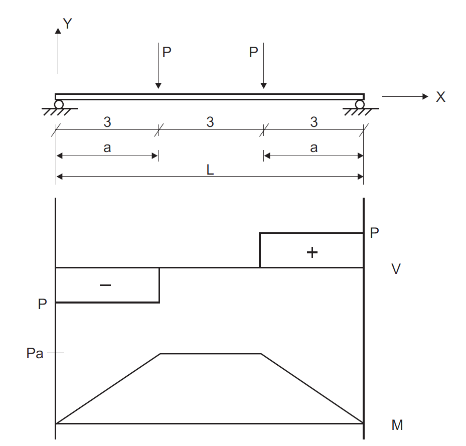
Figure 1: Simply supported beam with two equal concentrated loads (distance in units of meters).
The FLAC3D model contains 144 shell elements and 88 nodes, as shown in Figure 2. We utilize a cross-diagonal mesh pattern to ensure symmetric response, and we utilize a DKT plate bending finite element because this is a small-strain, plate-bending problem. The same results would be produced if we used either of the shell finite elements, because no membrane loading occurs. We set the Young’s modulus and Poisson’s ratio equal to 200 GPa and 0, respectively. We set the shell thickness equal to 0.133887 m to produce a second moment of inertia, \(I\), equal to 200 \(\times\) 10-6 m4. Boundary conditions consist of simple supports at the beam ends, and two point loads, each of which is 10,000 N. The point loads are distributed to the four nodes along each load line based on tributary length associated with each node. Thus, the inner nodes carry twice the load of the outer nodes.
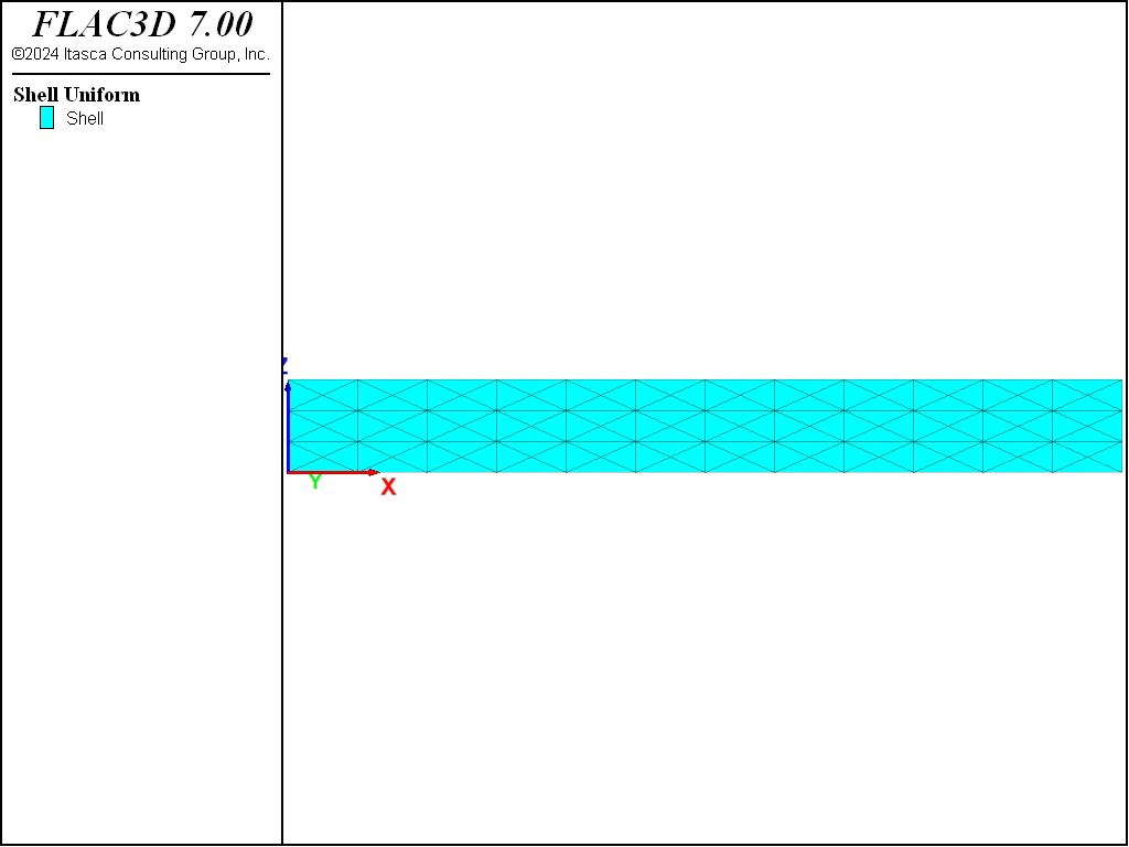
Figure 2: FLAC3D model for simple beam problem modeled with shell elements.
The displacement field is shown in Figure 3. The maximum displacement occurs at the beam center and equals 6.469 \(\times\) 10-3 m, which corresponds exactly with the theoretical value.
An alternative means of visualizing the displacement field for a small-strain simulation is to use the Shell plot item and specify a nonzero value for the deformation factor. Figure 4 shows both the undeformed and the deformed shape by adding two Shell plot items to the view and specifying deformation factors of zero and 100, respectively.
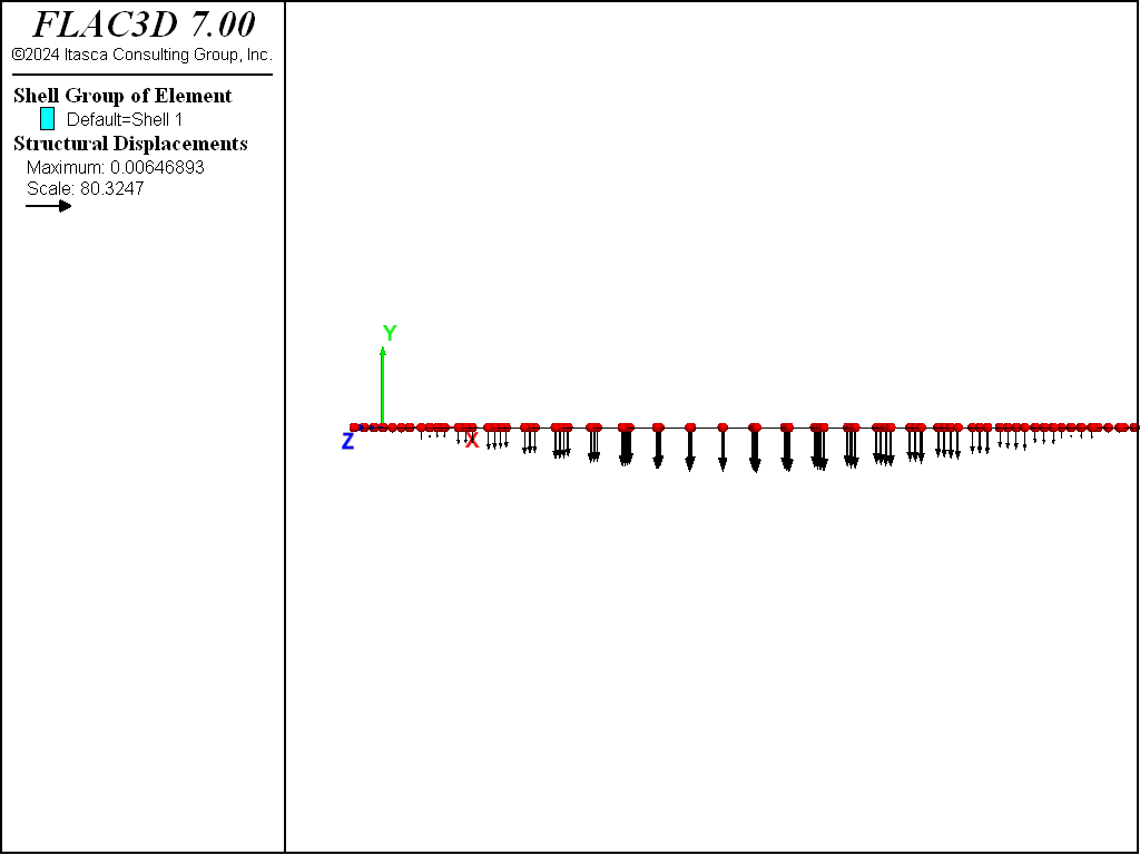
Figure 3: Displacement field of simple beam modeled with shell elements.
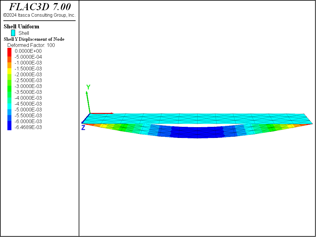
Figure 4: Deformed (factor of 100) and undeformed shapes of simple beam modeled with shell elements.
Figure 5 and Figure 6 show the shear force and moment distributions. Based on this scale, they correspond with the theoretical solutions. These plot items display these quantities in the surface coordinate system that is specified with the “Surf X” attribute, set such that the surface \(x\)-direction corresponds with the global \(x\)-direction, the surface \(y\)-direction corresponds with the global \(z\)-direction, and the surface \(z\)-direction corresponds with the negative global \(y\)-direction. The sign convention for these stress resultants is shown here. We see that positive \(M_x\) corresponds with stretching of the fibers in the positive \(z\)-direction of the surface, and positive \(Q_x\) corresponds with shear forces acting in the positive \(z\)-direction of the positive \(x\)-directed surface.
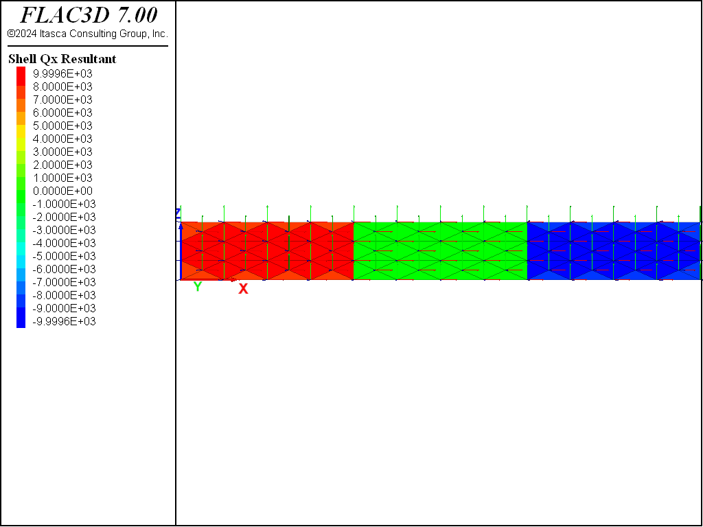
Figure 5: Shear force distribution in simple beam modeled with shell elements.
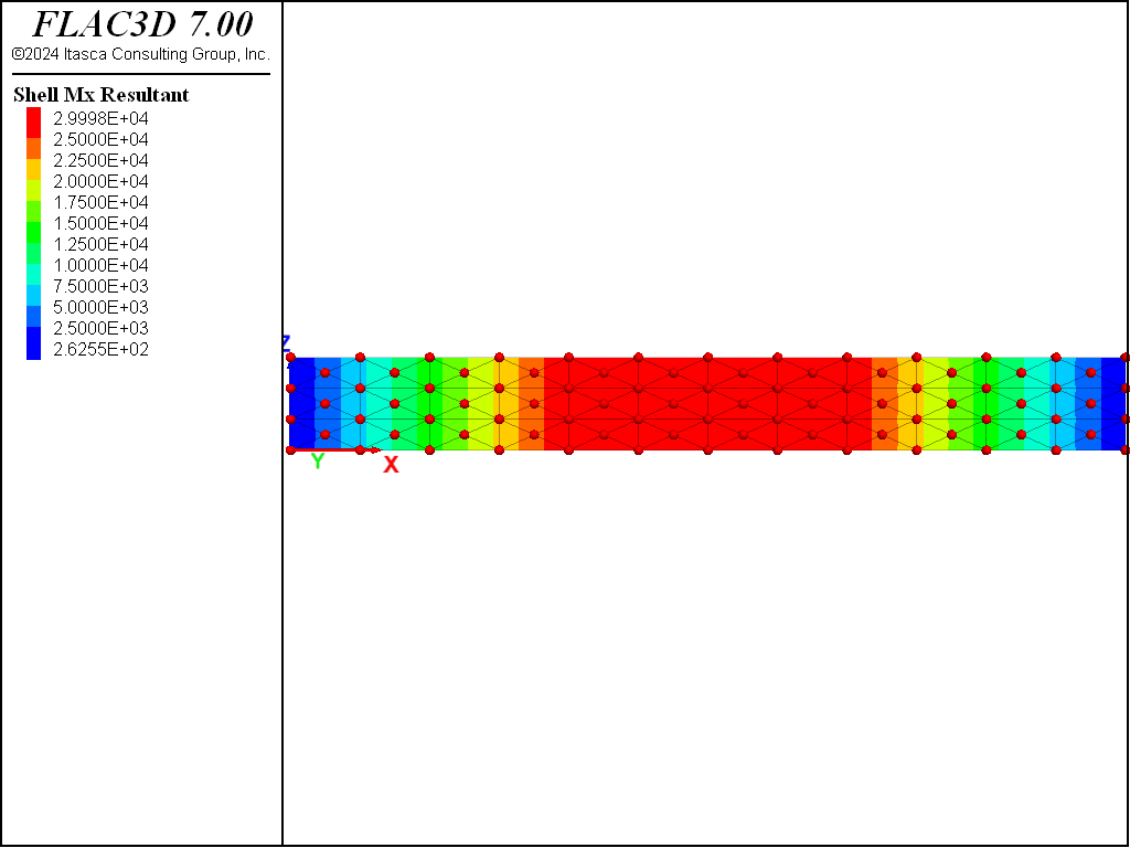
Figure 6: Moment distribution in simple beam modeled with shell elements.
A closer examination of the shear force and moment distributions in the left third of the beam is provided in Figure 8 and Figure 7. The moment distribution is constant across the depth and varies linearly from zero at the support to 3 \(\times\) 104 at the third point, which corresponds exactly with the theoretical solution. The shear distribution is not constant across the depth. It has the correct value away from the edges, but deviates from the beam-theory solution along the edges.
At \(x\) =1.5 away from the edge, the values of \(Q_x\) and \(M_x\) are found to be 1.0 \(\times\) 104 and 1.5 x 10⁴, respectively, which correspond exactly with the theoretical values. At \(x\) =1.5 near the edge, the values of \(Q_x\) and \(M_x\) are found to be 9.25 \(\times\) 103 and 1.5 \(\times\) 104, respectively. We see that there is an error of 7.5% in the value of shear force along the edge. This deviation from the beam-theory solution arises from the nonzero value of \(M_{xy}\) that develops at the nodes along the edge (see Figure 8).
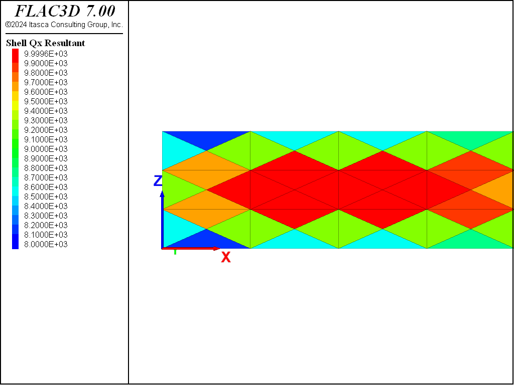
Figure 7: Shear force distribution in left third of simple beam modeled with shell elements.
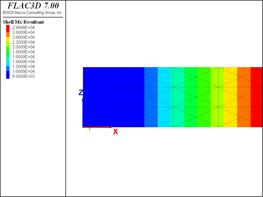
Figure 8: Moment distribution in left third of simple beam modeled with shell elements.
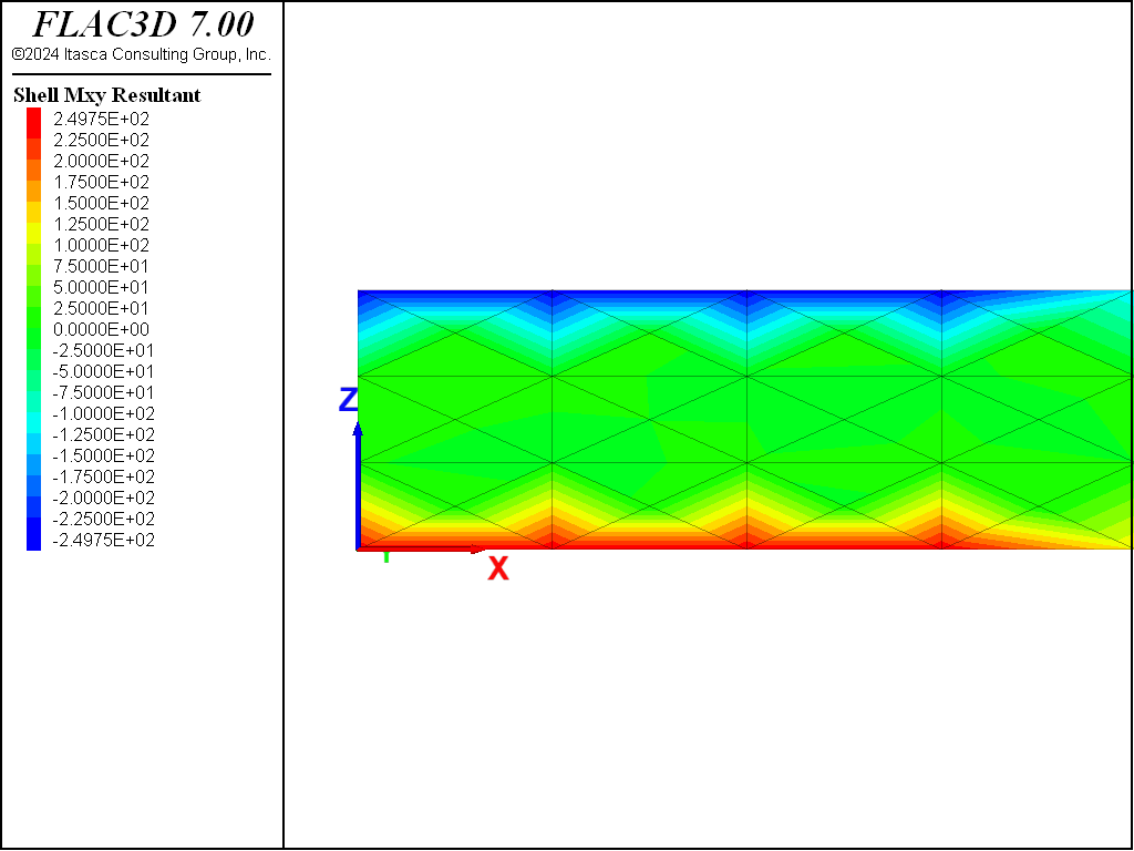
Figure 9: Twisting moment distribution in left third of simple beam modeled with shell elements.
The stress-recovery procedure smooths bending and membrane resultants at the nodes and then uses
the bending resultants to compute the constant value of transverse-shear resultants within each
shell element. The best accuracy is obtained by smoothing these values over each surface patch
for which the stresses will vary continuously. In this problem, when we compute stresses using
the structure shell recover command, by default, stresses are recovered, and thus
smoothed, for all shell elements in the model. The structure shell history
resultant-qx command, however, only recovers stresses for the particular element
identified; therefore, smoothing does not occur. In this problem, we sampled a history of
\(Q_x\) in one element using the command
struct shell history resultant-qx surface-x (1,0,0) position (1.625,0,0.5)
A plot of this quantity is shown in Figure 10, where we see that the
value does not equal the value of 1.0 \(\times\) 104, which we obtained above from
the plot item and from the structure shell recover resultants command. For this problem,
the smoothing process is necessary to produce good values of \(Q_x\).
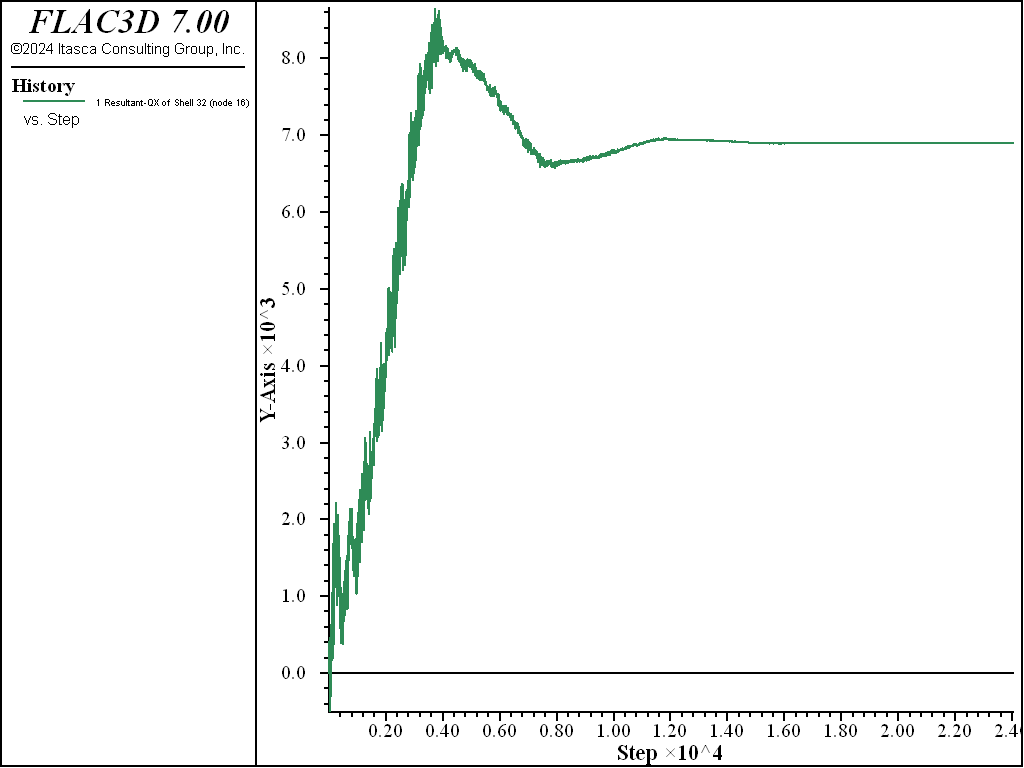
Figure 10: Evolution of shear force at centroid of a shell element (computed with no nodal smoothing).
Reference
Ugural, A. C. Stresses in Plates and Shells. New York: McGraw-Hill Publishing Company Inc. (1981).
Data File
ConcentratedLoads.dat
model new
model large-strain off
model title "Simple Beam (modeled using shell elements)"
; Create shell elements and assign material properties
struct shell create by-quadrilateral (0,0,0) (9,0,0) (9,0,1) (0,0,1) ...
                    size=(12,3) cross-diagonal element-type=dkt
struct shell property isotropic=(2e11, 0.0) thickness=0.133887
; Boundary conditions
struct node fix velocity-x velocity-y rotation-x rotation-y ...
                range position-x 0.0 ; support at left end - hinge
struct node fix velocity-y rotation-x rotation-y range position-x 9.0
                                      ; support at right end - roller
struct node fix velocity-z rotation-x rotation-y
           ; restrict non-beam deformation modes
; Applied loads
struct node apply force-edge (0,-1e4,0) range union position-x=3 position-x 6
; History
history interval 1
struct shell history resultant-qx surface-x (1,0,0) position (1.625,0,0.5)
; Solve to equilibrium
model solve ratio-local 1e-6
model save 'ConcentratedLoads'
| Was this helpful? ... | PFC © 2021, Itasca | Updated: Feb 25, 2024 |