
Dynamic Input Wizard
An illustrative use of the Dynamic Input Wizard (accessible from the menu ) is presented here.
A seismic loading corresponding to data from the 1987 Loma Prieta earthquake in California is used. The input record (i.e., the upward-propagating motion from the deconvolution analysis; SHAKE-91 is used in this example to estimate the appropriate motion at depth corresponding to the target (surface) motion) is stored in a file named “ACC DECONV.HIS”. The estimated peak acceleration in the input is approximately 5.8 ft/sec2.
[CS: original first paragraphs from FLAC altered to allow omission of first FLAC figure]
Step 1: Import Data File into the Wizard
To import the upward-propagating motion from the deconvolution analysis, the “file open” (yellow folder) button is pressed. The input file, “ACC_DECONV.HIS” in this case, is chosen and the “Select” button is pressed ( , see the image below). The file format “history” is chosen, “Acceleration” is set as the ground motion type, and imperial units (ft/s2) are selected. The “Next” button is pressed to move on to filtering.
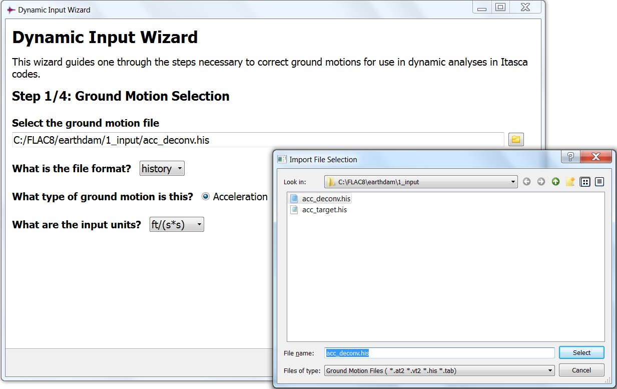
Figure 1: Import input into the wizard
Step 2: Filtering
The acceleration input record is integrated to produce a velocity record, which is then integrated again to get a displacement record. Those records are shown on the left section of the window.
A fast Fourier transform (FFT) analysis of the input acceleration record results in an amplitude spectrum as shown here:

Figure 2: Original input records, amplitude spectrum and filter
This figure indicates that the dominant frequency is approximately 1 Hz, the highest frequency component is less than 10 Hz, and the majority of the frequencies are less than 5 Hz. Most energy of the input is contained in lower frequency components. A Butterworth-type low-pass filter with a cutoff frequency of 5 Hz is applied to remove the frequency components above 5 Hz. The input records are updated after the circular green “Start” button (  ) is pressed, as shown below.
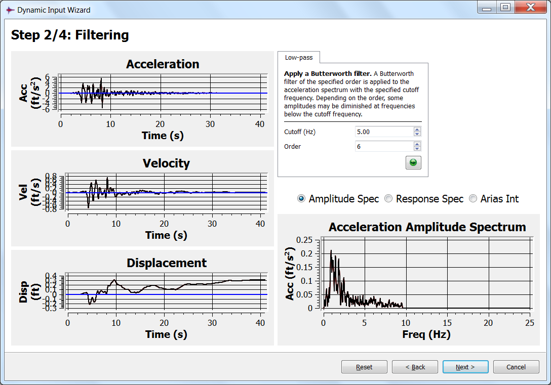
Figure 3: Filtered input records, amplitude spectrum
Step 3: Baseline Correction
The baseline correction window will appear after pressing the “Next” button shown in the image above. Four tabbed panes are provided to perform baseline correction. First press the Mean tab to remove the mean acceleration. This may not be necessary if the ground motion has been corrected. Next, remove the displacement drift via a low-frequency sinusoid function. The final displacement drift is found to be approximately 0.3 ft as shown below.
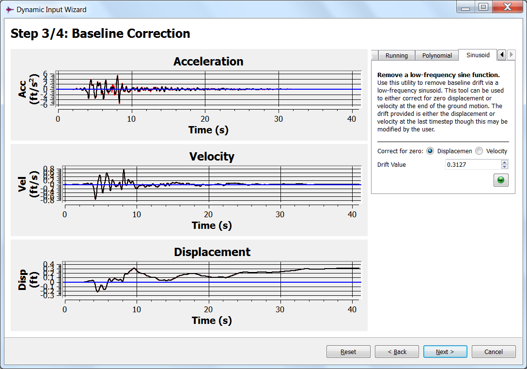
Figure 4: Waveform before baseline correction
By pressing the “Start” button ( ), the drift is removed and the final displacement is corrected to zero, as shown below.
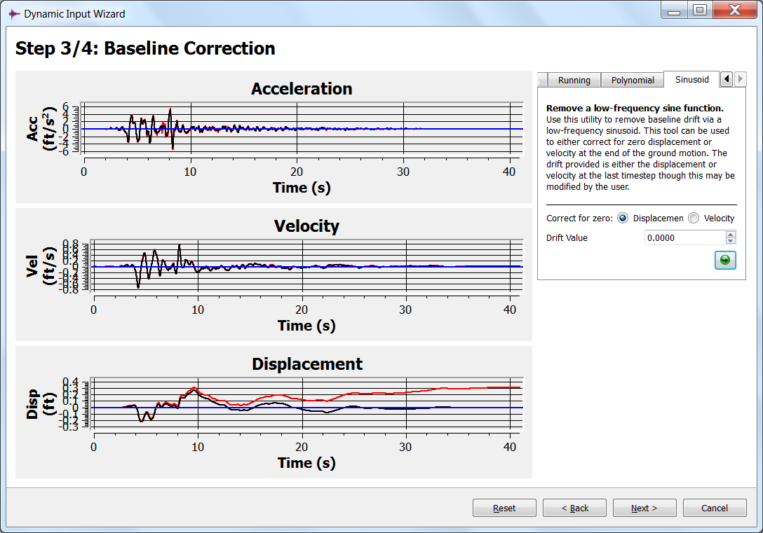
Figure 5: Waveform after baseline correction
Step 4: Export Data for Dynamic Analysis
The processed data can be saved by pressing the “save” button. This opens the “Export File Selection” dialog; in this case, the file is named “INPUT.TAB” and “Select” is pressed. “Velocity” is chosen as the motion type for export, and the output is set to “Table”. The Export button is pressed to export the data (see figure below for illustration).
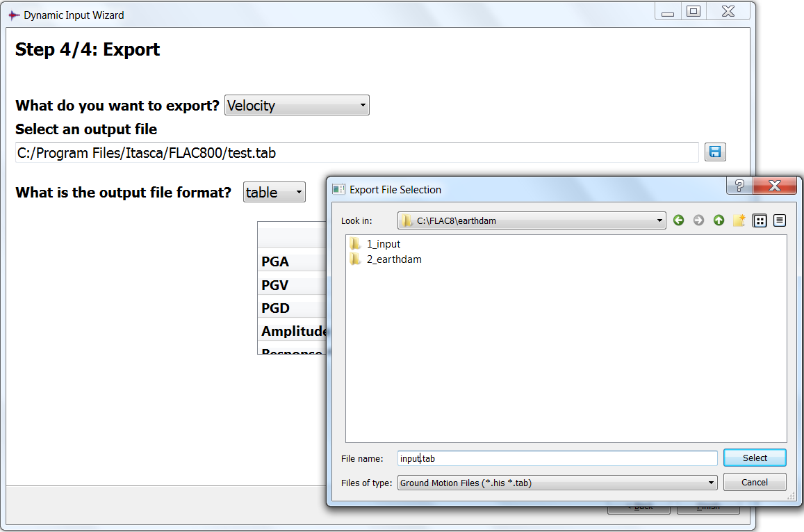
Figure 6: Save processed velocity in a table
| Was this helpful? ... | PFC © 2021, Itasca | Updated: Feb 25, 2024 |