
Slip Induced by Harmonic Shear Wave
Note
The project file for this example is available to be viewed/run in FLAC3D.[1] The main data files are shown at the end of this example. The remaining data files can be found in the project.
This problem concerns the effects of a planar discontinuity on the propagation of an incident shear wave. Two homogeneous, isotropic, semi-infinite elastic regions, separated by a planar discontinuity with a limited shear strength, are shown in Figure 1. A normally incident, plane harmonic, shear wave will cause slip at the discontinuity, resulting in frictional energy dissipation. Thus, the energy will be reflected, transmitted and absorbed at the discontinuity. The problem is modeled with FLAC3D, and the results are used to determine the coefficients of transmission, reflection, and absorption. These coefficients are compared with ones given by an analytical solution (Miller 1978).
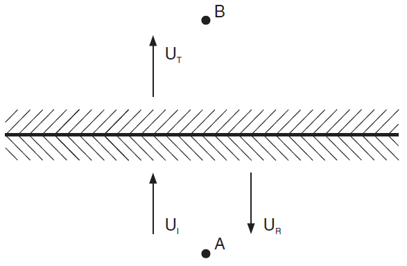
Figure 1: Transmission and reflection of incident harmonic wave at a discontinuity.
The coefficients of reflection (\(R\)), transmission (\(T\)), and absorption (\(A\)) given by Miller (1978) for the case of uniform material are
where \(E_I\), \(E_T\), and \(E_R\) represent the energy flux per unit area per cycle of oscillation associated with the incident, transmitted, and reflected waves, respectively. The coefficient \(A\) is a measure of the energy absorbed at the discontinuity. The energy flux \(E_I\) is given by
| where: | \(T\) | = | \((2 \pi)\thinspace /\thinspace \omega\) = the period for the incident wave; |
| \(\sigma_s\) | = | shear stress; | |
| \(v_s\) | = | particle velocity in the \(x\)-direction; and | |
| \(\omega\) | = | frequency of incident wave (radian/sec). |
For elastic media,
Hence,
in which \(c\) is the velocity of the propagating shear wave.
The energy flux of the incident wave, \(E_I\), is evaluated at point A (see Figure 1) for no slip at the discontinuity. The energy flux of the transmitted wave, \(E_T\), is evaluated at point B for the case of slip at the discontinuity. The energy flux of the reflected wave, \(E_R\), is calculated by determining the difference of velocities in two cases: slip and no slip.
Figure 2 shows the numerical model, which consists of two sub-grids (each with fifteen zones in the \(z\)-direction, two zones in the \(x\)-direction, and one zone in the \(y\)-direction) connected by an interface, EF, which has high stiffness and simulates the discontinuity. The conditions used are as follows.
Boundary Conditions
- Nonreflecting viscous boundaries are located at GH and CD.
- Vertical motion is prevented along lateral boundaries GC and DH.
- All gridpoints are fixed in the \(y\)-direction (i.e., a condition of plane strain is enforced).
Loading Conditions
- Shear stresses corresponding to the incident wave are applied along CD.
- The maximum stress of the incident wave is 1 MPa, and the frequency is 1 Hz.
Material Conditions
elastic media
\(\rho\) = 2.65 × 10³ kg/m3
\(K\) = 16,667 MPa
\(G\) = 10,000 MPa
interface
\(k_{x}\) = \(k_{s}\) = 10,000 MPa/m
\(C\) = cohesion = 2.5 MPa for no-slip case; = 0.5, 0.1, 0.02 MPa for slip case
Note that the magnitude of the incident wave must be doubled in the numerical model to account for the simultaneous presence of the nonreflecting boundary (see Application of Dynamic Input).
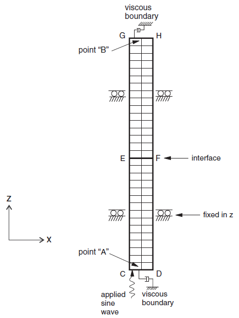
Figure 2: Problem geometry and boundary conditions for the problem of slip induced by harmonic shear wave.
Four different cases are run at an interface cohesion of 2.5, 0.5, 0.1, and 0.02 MPa, respectively. The \(x\)-velocity histories at the top and bottom of the model (point A and B) are stored in tables xvelbotN and xveltopN, where N is the case from 1 to 4. At the start of each case, the previous model is reset without deleting the tables storing results by deleting all zones and histories, and resetting the total dynamic time to 0.
The cohesion in case 1 is high enough to ensure a fully elastic response, and Figure 3 shows the time variation of shear stress near points A and B. From the amplitude of the stress histories at A and B, it is clear that there is perfect transmission of the wave across the discontinuity. It is also clear from Figure 3 that the viscous boundary condition provides perfect absorption of normally incident waves.
The recorded shear stresses at points A and B for cases 2, 3, and 4 are shown in Figures 4, 5, and 6, respectively. The peak stress at point A is the superposition of the incident wave and the wave reflected from the slipping discontinuity. It can be seen in Figures 4 through 6 that the shear stress of point B is limited by the discontinuity strength.
After all cases are run, the energy flux and coefficients \(R\), \(T\), and \(A\) are computed by FISH function energy and written to the tables f3_A, f3_R, and f3_t. It was determined that at least five cycles of the input wave were necessary before the computed coefficients settled down to steady-state values. Even then, there is a periodic fluctuation in the values. In order to obtain mean values, the coefficient values were averaged over the final 100 timesteps. Figure 7 compares the numerical results with the exact solution for the coefficients for three values of the dimensionless parameter.
| where: | \(\tau_{s}\) | = | discontinuity cohesion; |
| \(U\) | = | displacement amplitude of the incident wave; | |
| \(\gamma\) | = | \(\sqrt{\rho\ G}\); and | |
| \(\omega\) | = | frequency of incident wave (1 Hz). |
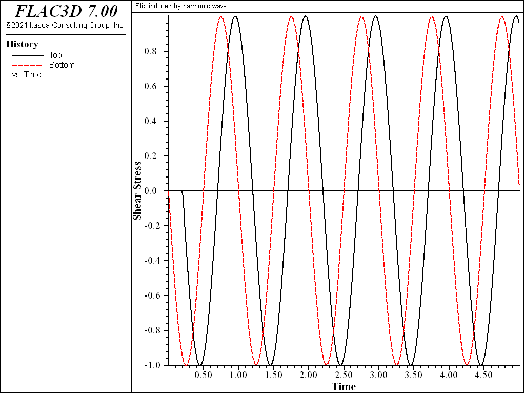
Figure 3: Time variation of shear stress at points A and B for elastic discontinuity (cohesion = 2.5 MPa).
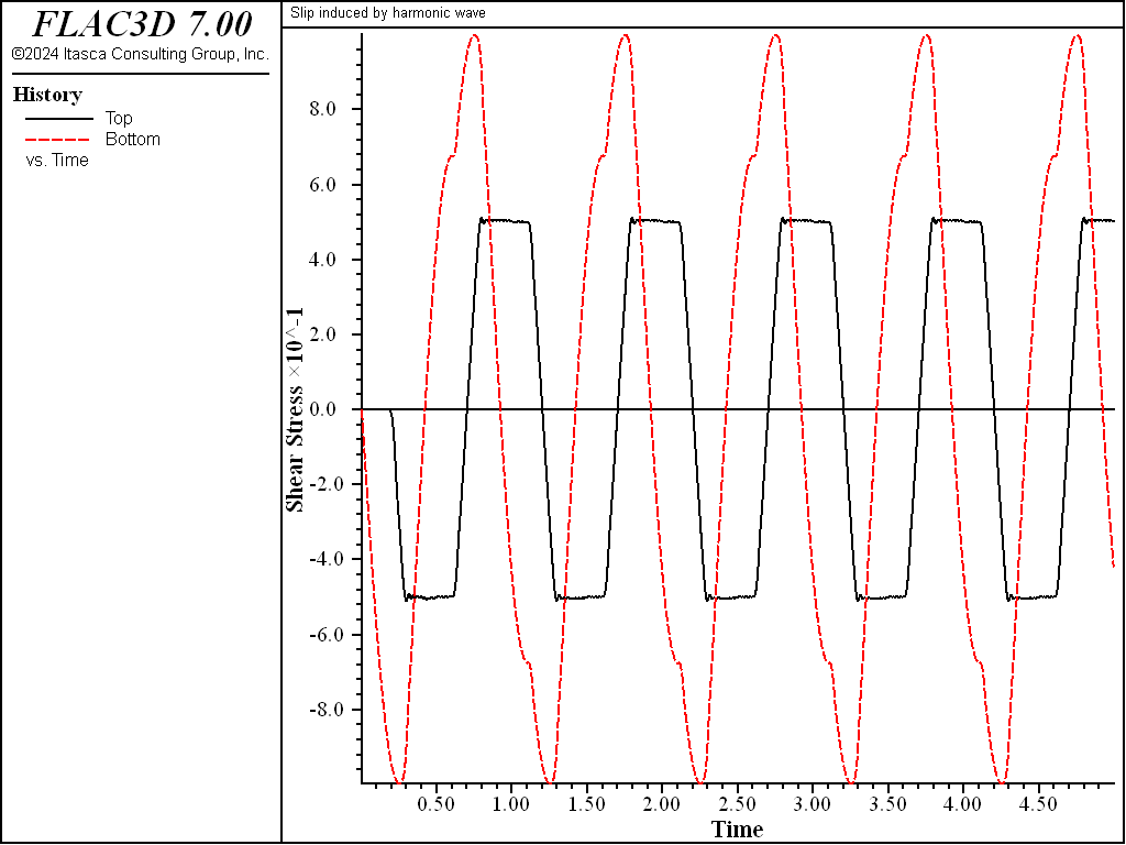
Figure 4: Time variation of shear stress at points A and B for slipping discontinuity (cohesion = 0.5 MPa).
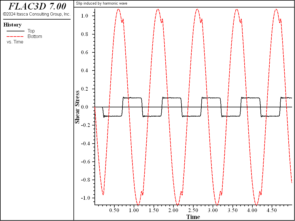
Figure 5: Time variation of shear stress at points A and B for slipping discontinuity (cohesion = 0.1 MPa).
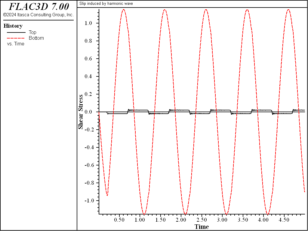
Figure 6: Time variation of shear stress at points A and B for slipping discontinuity (cohesion = 0.02 MPa).
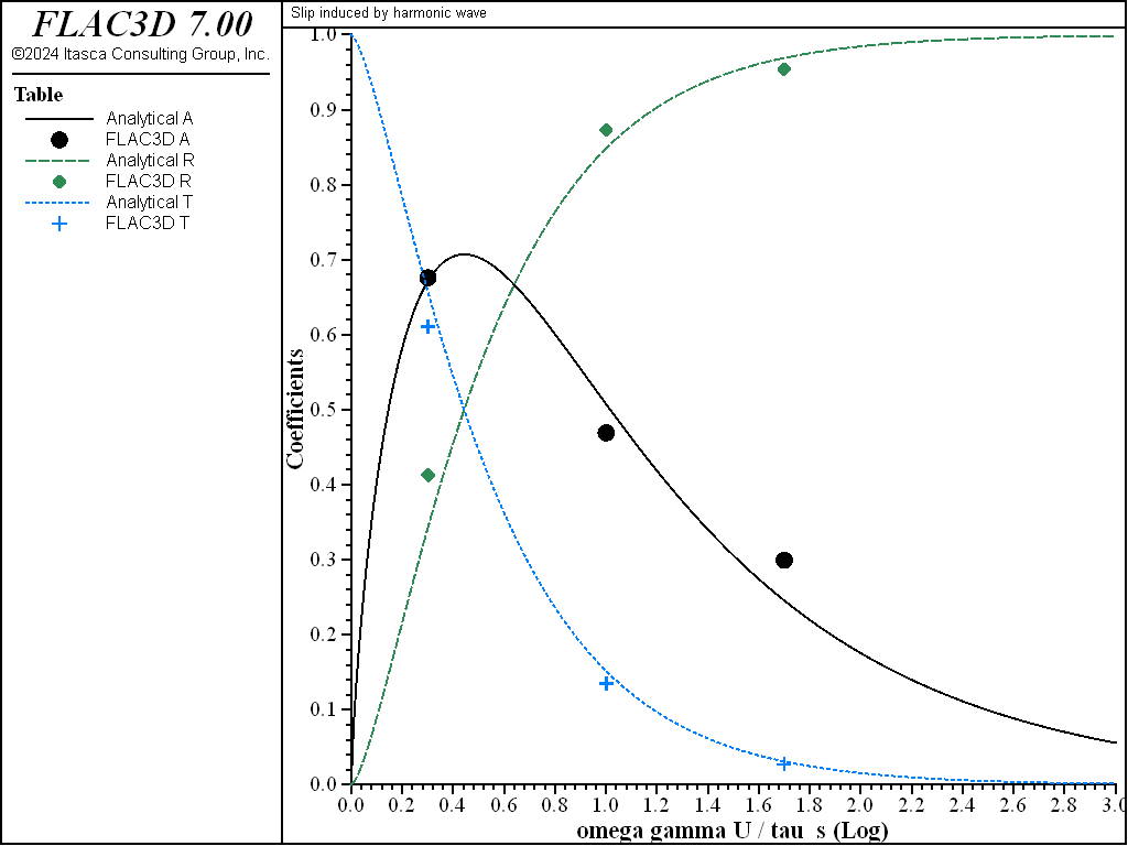
Figure 7: Comparison of transmission, reflection, and absorption coefficients (points denote FLAC3D results.
The displacement amplitude for the incident wave (\(U\)) was obtained by monitoring the horizontal displacement at point A for non-slipping discontinuities. As can be seen, the FLAC3D results agree well with the analytical solution.
References
Miller, R. K. “The Effects of Boundary Friction on the Propagation of Elastic Waves,” Bull. Seismic. Assoc. America, 68, 987-998 (1978).
Data Files
SlipInducedHarmonicShearWave.dat
;---------------------------------------------------------------------
; script file for dynamic problem 'Slip induced by harmonic wave'
;---------------------------------------------------------------------
model new
fish automatic-create off
model title "Slip induced by harmonic wave"
model configure dynamic

; Define simple FISH function for applied stress, sine wave
fish define fsin
    return math.sin(2.0*math.pi*dynamic.time.total)
end

[global coh_list = list.sequence(2.5,0.5,0.1,0.02)]
            ; Four cases, cohesion from 2.5 to 0.02
fish define runAllCases
    loop local casenum (1,list.size(coh_list))
        local cohesion = coh_list(casenum)
        system.command("program call 'common'")
    end_loop
end
[runAllCases]
model save 'final'
common.dat
model large-strain off
; Clear any previous model
zone delete
history delete
model dynamic time-total 0

; Create zones
zone create brick point 0 (0,0,-200) point 1 add (30,0,0) ...
                  point 3 add (0,0,200) point 2 add (0,15,0) ...
                  size 2 1 15 group 'Bottom'
zone create brick point 0 (0,0,   0) point 1 add (30,0,0) ...
                  point 3 add (0,0,200) point 2 add (0,15,0) ...
                  size 2 1 15 group 'Top'

; Assign constitutive model and properties
zone cmodel assign elastic
zone property bulk 16667 shear=10000.0 density=0.00265

; Create interface, and assign interface properties
zone interface 'disc' create by-face separate ...
                                     range group 'Bottom' group 'Top'
zone interface 'disc' node property stiffness-normal 10000 ...
                                    stiffness-shear 10000 ...
                                    cohesion [cohesion] ...
                                    friction 0.0 ...
                                    tension 1e6 ...
                                    bonded-slip on
; Assign boundary conditions
zone gridpoint fix velocity-y
zone gridpoint fix velocity-z range union position-x 0 position-x 30
zone face apply quiet range union position-z -200 position-z 200
zone face apply stress-dip 2 fish fsin range position-z -200

; Take histories
history interval 10
model history name='time'     dynamic time-total
zone  history name='xvelbot'  velocity-x     position (15,0,-200) ; A
zone  history name='xveltop'  velocity-x     position (15,0, 200) ; B
zone  history name='sxzbot'   stress-xz      position (15,0,-200) ; A
zone  history name='sxztop'   stress-xz      position (15,0, 200) ; B
zone  history name='xdispbot' displacement-x position (15,0,-200) ; A

; Solve model to time 5, and save
model solve time-total 5
model save ['case'+string(casenum)]

; Export Velocity histories to tables
history export 'xvelbot'  vs 'time' table ['xvelbot'+string(casenum)]
history export 'xveltop'  vs 'time' table ['xveltop'+string(casenum)]
history export 'xdispbot' vs 'time' table ['xdisptop'+string(casenum)]
Endnotes
| [1] | To view this project in FLAC3D, use the program menu.
⮡ FLAC |
⇐ Comparison of FLAC3D to SHAKE for a Layered, Nonlinear-Elastic Soil Deposit | Hollow Sphere Subject to an Internal Blast ⇒
| Was this helpful? ... | PFC © 2021, Itasca | Updated: Feb 25, 2024 |