
Axial and Lateral Loading of a Concrete Pile
Problem Statement
Note
To view this project in FLAC3D, use the menu command . Choose “ExampleApplications/ ConcretePile” and select “ConcretePile.prj” to load. The main data files used are shown at the end of this example. The remaining data files can be found in the project.
The load-deflection response of a single concrete pile foundation is calculated for loading in both the axial and lateral directions. The pile is first subjected to an axial load of 100 kN, and then the top of the pile is moved horizontally for a maximum displacement of 4 cm. The relation of the axial loading to the ultimate bearing capacity of the pile is determined, and a lateral load-deflection curve is calculated.
The pile is 0.6 m in diameter, 5 m in length, and is embedded in a homogeneous clay layer. The groundwater surface is at a depth of 5.5 m. The properties of the concrete pile and the clay are summarized in Table 1.
| Concrete Pile | Clay | |
|---|---|---|
| Dry density | 2500 kg/m3 | 1230 kg/m3 |
| Wet density | - | 1550 kg/m3 |
| Elastic Properties: | ||
| Young’s modulus | 25.0 GPa | 100.0 MPa |
| Poisson’s ratio | 0.20 | 0.30 |
| Bulk modulus | 13.9 GPa | 83.33 MPa |
| Shear modulus | 10.4 GPa | 38.46 MPa |
| Strength Properties: | ||
| Cohesion | - | 30 kPa |
| Friction angle | - | 0.0 |
Modeling Procedure
A vertical plane through the pile axis is a plane of symmetry for this analysis. The coordinate axes for the FLAC3D model are located with the origin at the top of the pile, and the \(z\)-axis oriented along the pile axis and upward. The model grid is shown in Figure 1. The top of the model, at \(z\) = 0, is a free surface. The base of the model, at \(z\) = -8 m, is fixed in the \(z\)-direction, and roller boundaries are imposed on the sides of the model at \(|x|\) = 8 m and \(y\) = 8 m.
The axial-bearing capacity of a pile is a function of the skin friction resistance along the pile shaft and the end-bearing capacity at the pile tip. The skin friction resistance is modeled by placing an interface between the pile walls and the clay. The friction and cohesion properties of the interface represent the frictional resistance between the concrete and the clay. For this example, a friction angle of 20° and a cohesion of 30 kPa are assumed for the interface properties. A second interface is placed between the pile tip and the clay.
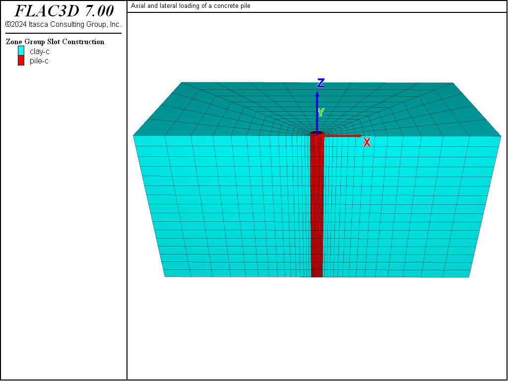
Figure 1: FLAC3D grid for vertical and lateral loading of a concrete pile in clay.
For optimum performance, two separate interfaces are used—one at the pile wall and one at the pile base. The zone faces are separated in a previous command so that the gridpoints common to both will be separated as well.
The model is first brought to an equilibrium stress-state under gravitational loading before the installation of the pile. A horizontal water table is created at \(z\) = -5.5 m, and the wet density of the clay is assigned to the zones below the water table. In the next stage of analysis, the model is brought into equilibrium after the installation of the pile. The installation is modeled by changing the properties of the pile zones from the properties representing the clay material to those representing the concrete pile material. The vertical stress-distribution at the equilibrium state, including the weight of the pile, is shown in Figure 2.
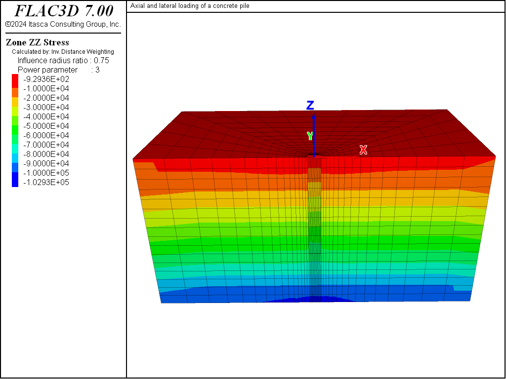
Figure 2: Contours of vertical stress at the initial stress-state, including the weight of the pile.
The ultimate bearing capacity of the pile in the axial direction is calculated by applying a vertical velocity at the top of the pile. The velocity is applied by means of a “ramp” (i.e., the boundary condition is increased linearly from zero to the desired value). This is particularly helpful for this problem because of the large contrast in stiffnesses between the concrete and the clay, which produces a large contrast in natural periods of this model. Many thousands of timesteps are required to propagate a loading through the model, because the critical timestep is controlled by the high stiffness of the concrete. If the velocity is applied suddenly, the inertial effects will dominate initially and make it more difficult to identify the steady-state response of the system.
The table ramp is used to apply the velocity to the pile top gridpoints. The FISH function vert�_load calculates the axial stress at the top of the pile and stores the value as a history. For efficiency, the gridpoints on the cap surface are stored in the symbol cap as a map. A plot of axial stress versus axial displacement at the pile top is shown in Figure 3, for the condition of the velocity applied as a ramp from 0.0 to 5x10⁻⁸ over 30,000 steps. Note that only a small amount of oscillation is observed initially in this response.
Combined damping is used for this stage of the analysis because this type of damping is more efficient at removing kinetic energy from the model for the prescribed loading condition. For the applied velocity loading, the velocity components of most of the gridpoints will not change sign. Local damping is not effective for this situation because the mass-adjustment process depends on velocity sign-changes. (See the section on mechanical damping in the Theory and Background section.)
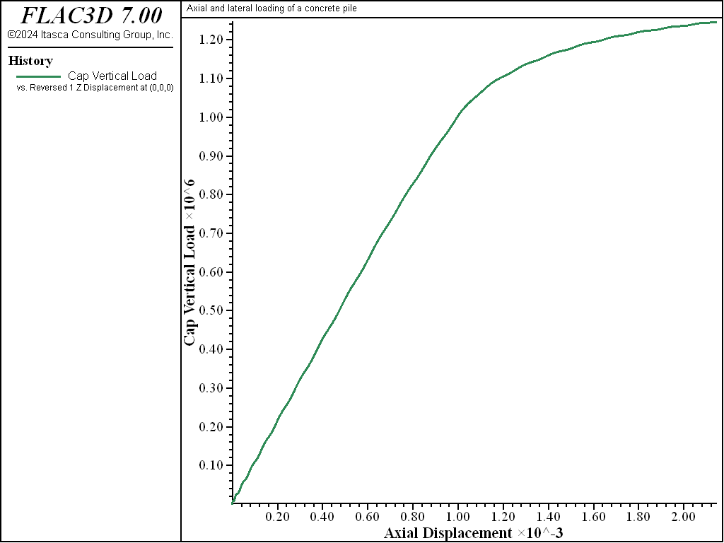
Figure 3: Axial stress versus axial displacement at pile top.
Figure 3 indicates that the ultimate bearing capacity of the pile is approximately 1.1 MPa. The ultimate capacity is a function of the pile-tip bearing and skin (friction) friction resistance. For example, if the interface cohesion is set to zero, then the only resistance is provided by the pile tip, and the ultimate capacity is calculated to be approximately 0.3 MPa. It is recommended that the calculated pile capacity be compared to field test results in order to determine the appropriate values to use for interface strength properties.
The analysis is repeated from the initial gravitational loading state to calculate the response to an axial loading of 100 kN. This loading is achieved by applying an axial stress of 0.354 MPa to the pile top. The applied stress is approximately a factor of 3 smaller than the ultimate axial capacity. For this loading, the pile top moves downward 0.33 mm.
After the model is brought to equilibrium for the 100 kN axial loading, the pile top is then moved laterally for a deflection of 4 cm. This is accomplished by applying a horizontal velocity at the pile top. A ramp loading is not used at this stage because the inertial effects are minor for loading in this direction. A horizontal velocity of 1x10⁻⁷ is applied to the pile cap.
The lateral force-deflection curve for the top of the pile is shown in Figure 4. The lateral load required to produce 4 cm of deflection is approximately 300 kN. The displacement of the pile and the plastic state of the soil at this stage are shown in Figure 5.
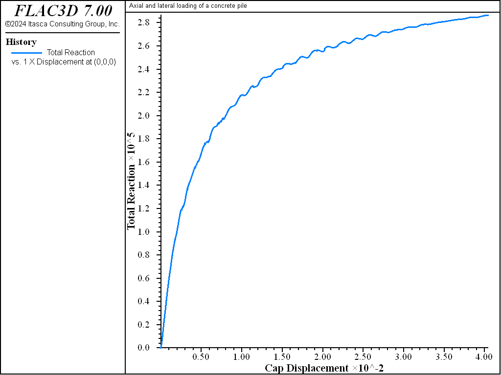
Figure 4: Lateral force versus lateral displacement at the pile top.
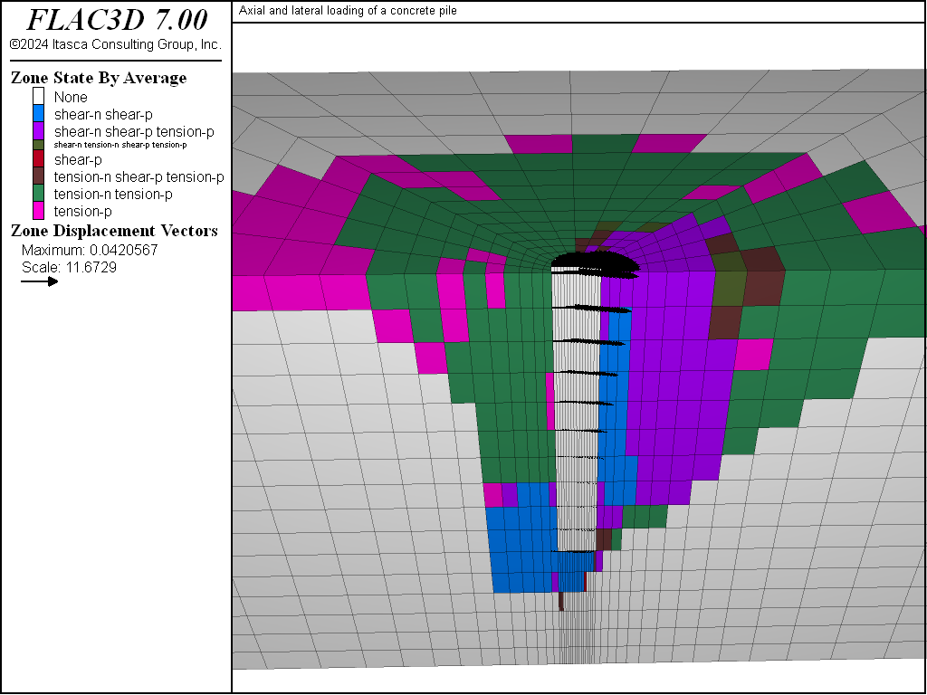
Figure 5: Pile displacement and plasticity state of soil at 4 cm lateral deflection.
A FISH function, tot�_reac in the file “p-y.dat” is used to monitor soil reaction along the pile as a function of lateral displacement. tot�_reac creates tables of soil reaction (\(p\)) versus lateral displacement (\(y\)) at different locations along the pile in order to generate \(p-y\) curves. Calculated \(p-y\) curves are shown in Figure 6.
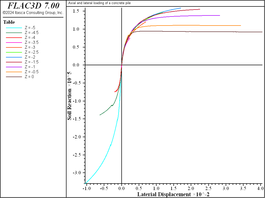
Figure 6: \(p-y\) curves at 11 equidistant points along the pile [soil reaction, p (N/m), versus lateral displacement, y (m)].
Data File
ConcretePile.dat
model new
model large-strain off
model title 'Axial and lateral loading of a concrete pile'
; create grid interactively from the extruder tool,
; exported to geometry.f3dat from State Record pane.
program call 'geometry' suppress
zone generate from-extruder
; Reflect the grid to get a 1/2 space instead of a 1/4 space
zone reflect dip-direction 270 dip 90
; Name intersections of things named in the two extruder views
zone group 'clay' range group 'clay-c' or 'clay-s' or 'wetclay-s'
zone group 'pile' range group 'pile-c' group 'pile-s' or 'remove-s'
zone group 'remove' range group 'remove-s' group 'pile-c' not ;
zone face group 'wall' internal range group 'wall-c' group 'pile'
zone face group 'base' internal range group 'base-s' group 'pile'
zone face skin ; Name far field boundaries
; Delete the area marked for removal
zone delete range group 'remove'
;
; setup interfaces - separate using ZONE SEPARATE
; all at once so common nodes are separated
zone separate by-face new-side group 'iwall' slot 'int' ...
     range group 'wall' or 'base'
; Want two different interfaces for proper normal direction at corner
zone interface 'side' create by-face range group 'wall' and 'iwall'
zone interface 'base' create by-face range group 'base' and 'iwall'
; Save initial geometric state
model save 'geometry'
;
; Initialize gravity, pore-pressures, density, and stres state
model gravity 10
; water table information
zone water density 1000
zone water plane origin (0,0,-5.5) normal (0,0,-1)
zone initialize density 1230
zone initialize density 1550 range group 'wetclay-s' ; Wet density
; assign properties to the soil and interfaces - temporarily remove pile cap
zone cmodel assign mohr-coulomb ...
     range group 'clay'
zone property bulk 8.333e7  shear 3.846e7  cohesion 30000 fric 0 ...
     range group 'clay'
zone cmodel assign elastic                 range group 'pile'
zone property bulk 8.333e7  shear 3.846e7  range group 'pile'
zone cmodel assign null                    range group 'remove-s'
zone interface node property stiffness-normal 1e8 ...
                             stiffness-shear 1e8 friction 20 cohesion 30000
; boundary and initial stress conditions
zone face apply velocity-normal 0 range group 'Bottom'
zone face apply velocity-normal 0 range group 'East' or 'West'
zone face apply velocity-normal 0 range group 'North' or 'South'
zone initialize-stress ratio 0.4286
zone interface node initialize-stresses
; Solve to initial equilibrium
zone ratio local
model solve ratio 1e-4
model save 'initial'
;
; install the pile
model restore 'initial'
zone cmodel assign elastic                          range group 'pile'
zone property bulk 13.9e9 shear 10.4e9 density 2500 range group 'pile'
model solve ratio 1e-4
model save 'install'
;
; vertical loading
zone initialize state 0
zone gridpoint initialize displacement (0,0,0)
zone gridpoint initialize velocity     (0,0,0)
table 'ramp' add ([global.step],0) ([global.step+30000],-5e-8) ...
      ([global.step+58000],-5e-8) ; Increase velocity applied to pile
                                  ; over 30,000 steps
zone face apply velocity-normal 1 table 'ramp' range group 'Top'
history interval 250
zone history name 'disp' displacement-z position (0,0,0)
program call 'load'
fish history name 'load' vert_load
zone mechanical damping combined
model step 58000
model save 'vertical-loading'
;
; vertical loading then lateral loading
model restore 'install'
zone initialize state 0
zone gridpoint initialize displacement (0,0,0)
zone gridpoint initialize velocity     (0,0,0)
zone face apply stress-zz [-1.0e5/(math.pi*0.3*0.3)] range group 'Top'
model solve ratio 1e-4
model save 'lateral-load-start'
; apply lateral loading as x-velocity on cap
zone initialize state 0
zone gridpoint initialize displacement (0,0,0)
zone gridpoint initialize velocity     (0,0,0)
zone face apply velocity-x 1e-7 range group 'Top'
zone history name 'disp' displacement-x position 0,0,0
; Calculate p-y curve for pile, when tot_reac is called
program call 'p-y' suppress
[make_pydata]        ; Generate p-y curve calculation data
[output_structure]   ; Sanity check of p-y curve data
fish history name 'load' tot_reac
model step 416500
model save 'lateral-load'
⇐ Prediction of Borehole Closure in a Salt Formation | Undrained Cylindrical Cavity Expansion in a Cam-Clay Medium ⇒
| Was this helpful? ... | PFC © 2021, Itasca | Updated: Feb 25, 2024 |