
Cylindrical Hole in an Infinite Mohr-Coulomb Material
Problem Statement
Note
To view this project in FLAC3D, use the menu command . Choose “VerificationProblems/CylinderInMohrCoulomb” and select “CylinderInMohrCoulomb.prj” to load. A representative sample of the data files used for hexahedral zones and associated flow is shown at the end of this example. The remaining data files can be found in the project.
Stresses and displacements are determined numerically for the case of a cylindrical hole in an infinite elasto-plastic material subjected to in-situ stresses. The material is assumed to be linearly elastic, perfectly plastic, with a failure surface defined by the Mohr-Coulomb criterion, and both associated (dilatancy = friction angle) and nonassociated (dilatancy = 0) flow rules are used. The results of the simulation are compared with an analytic solution.
This problem tests the Mohr-Coulomb plasticity model with plane-strain conditions imposed in FLAC3D.
The Mohr-Coulomb material is assigned several properties:
| shear modulus (\(G\)) | 2.8 GPa |
| bulk modulus (\(K\)) | 3.9 GPa |
| cohesion (\(c\)) | 3.45 MPa |
| friction angle (\(\phi\)) | 30° |
| dilation angle (\(\psi\)) | 0° and 30° |
The isotropic in-situ stress has a magnitude of -30 MPa, and the pressure inside the hole may be neglected. (As a convention, compressive stresses are negative.) The radius, \(a\), of the hole is small compared to the length of the cylinder, so that plane-strain conditions are applicable.
Closed-Form Solution
The analytic solution for this problem may be found in Salençon (1969). The yield zone radius, \(R_0\), may be expressed, in general terms, as
in which \(a\) is the hole radius, \(P_0\) is the absolute value of the in-situ isotropic stress, \(P_i\) is the pressure inside the hole (0 Pa, in this case), and
The radial stress at the elastic/plastic interface may be written as
The stresses in the plastic zone have the form
in which \(r\) is the distance from the hole axis.
The stresses in the elastic zone are
The displacements in the elastic region are given as
and, in the plastic region, as
in which
and
In these equations, \(\nu\) is Poisson’s ratio, \(\psi\) is the dilation angle and \(G\) is the shear modulus.
FLAC3D Model
For modeling purposes, the problem is defined by the domain sketched in Figure 1, where advantage has been taken of the quarter-symmetry geometry. A system of reference axes is selected, with orientation as indicated on the figure and origin located at the intersection of the hole axis with the front face of the domain. The far \(x\)- and \(z\)-boundaries are situated at a distance of five hole-diameters from the axis of the hole. The thickness of the domain is selected as one-tenth of the hole diameter.
The boundary conditions applied to this domain are sketched in Figure 2. The domain is discretized into one layer of 900 zones. The zones are organized in a radial pattern, as shown in Figure 3.
In the numerical simulation, the initial stress state (corresponding to \(P_0\) = 30 MPa) is applied throughout the domain first, and then the hole is removed.

Figure 1: Domain for FLAC3D simulation—quarter symmetry.
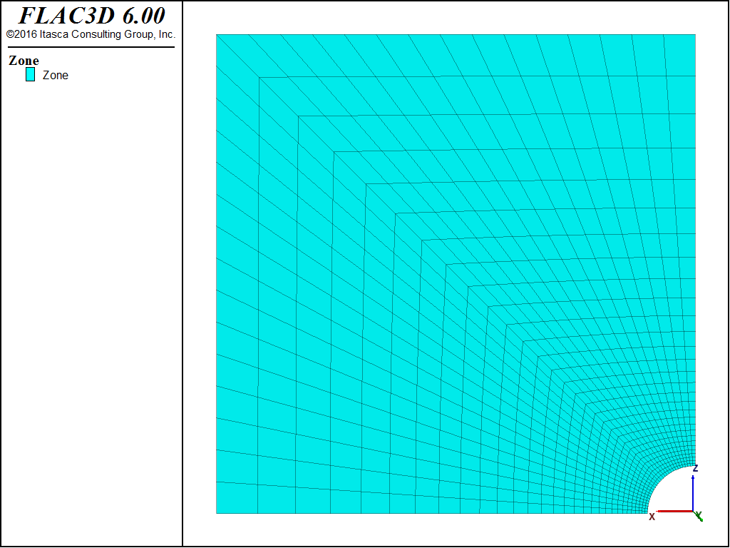
Figure 2: Boundary conditions for FLAC3D analysis—quarter symmetry.
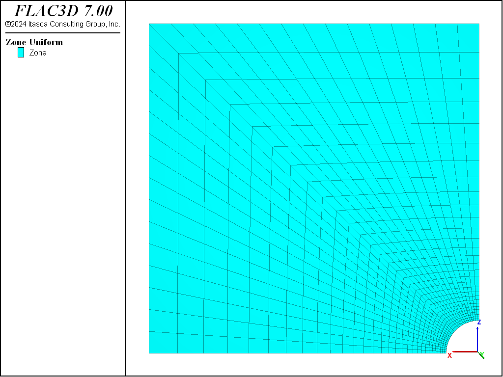
Figure 3: FLAC3D grid—quarter symmetry.
Results and Discussion
Figure 4 through Figure 7 show comparisons between FLAC3D results and the analytic solution along a radial line. Normalized stresses, \(-{\sigma}_r/P_0\) and \(-{\sigma}_{\theta}/P_0\), are plotted versus normalized radius, \(r/a\), in Figure 4 and Figure 5, while normalized displacements, \(-u_r/a\), are represented versus \(r/a\) in Figure 6 and Figure 7. Note that numerical stress values for the two flow rules cannot be differentiated on the graphs.
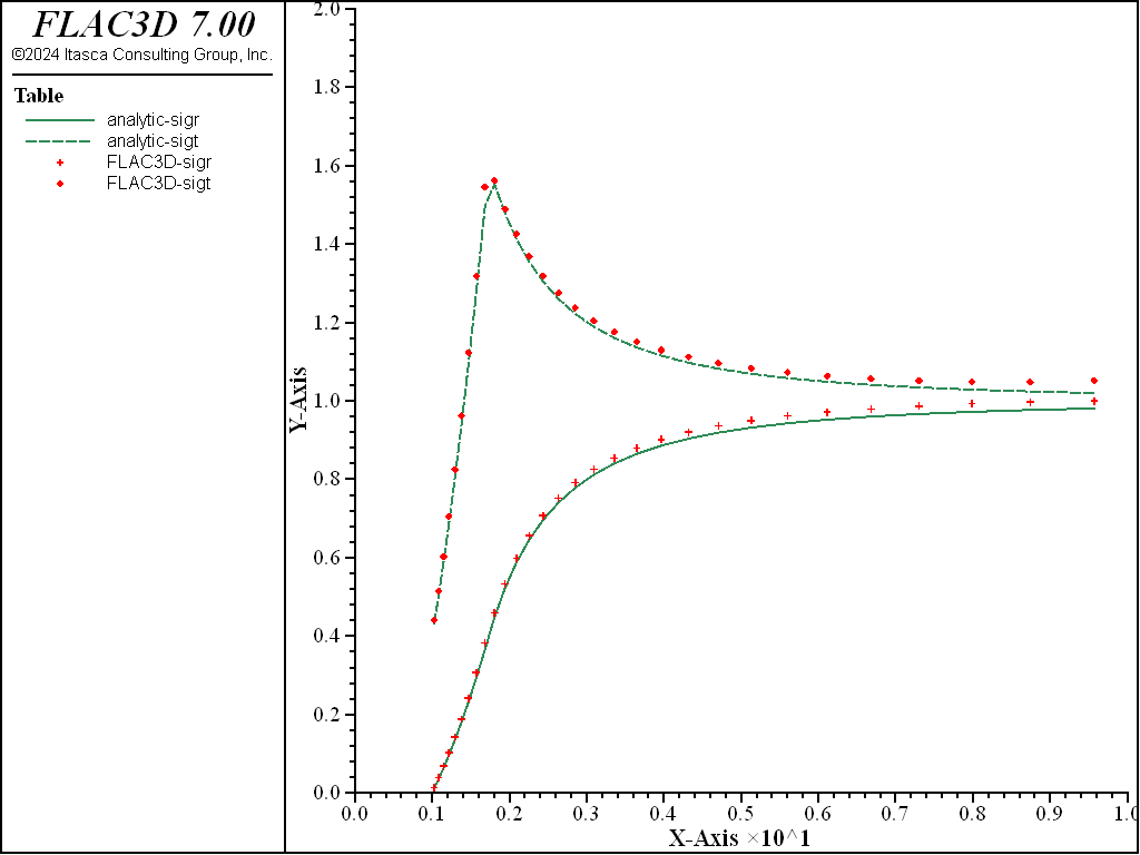
Figure 4: Stress solution comparison—associated (analytical values = lines; numerical values = crosses).
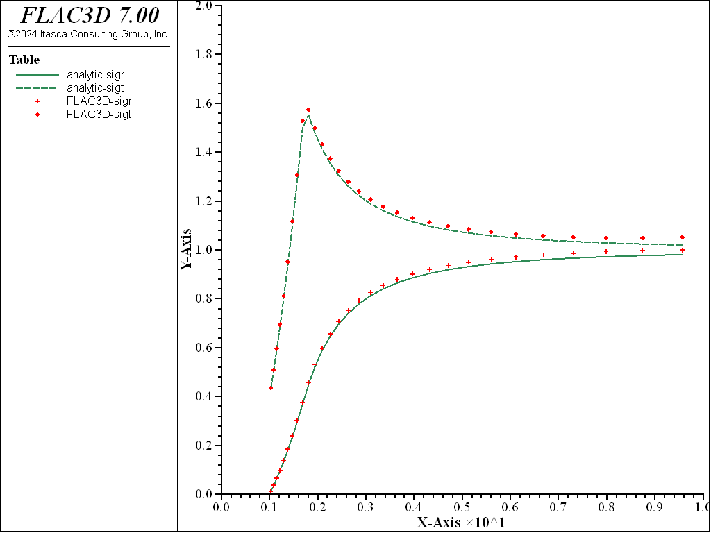
Figure 5: Stress solution comparison—nonassociated (analytical values = lines; numerical values = crosses).
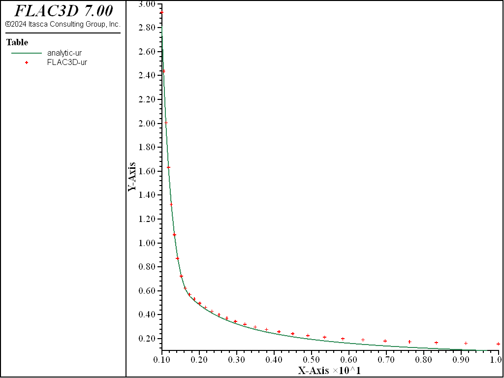
Figure 6: Radial displacement solution comparison—associated (analytical values = lines; numerical values = crosses).
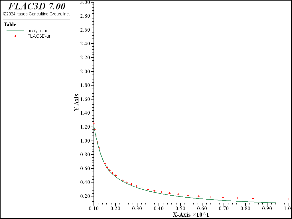
Figure 7: Radial displacement solution comparison—nonassociated (analytical values = lines; numerical values = crosses).
The average relative error on the stresses and displacements is less than 2.1% (except 4.6% for displacements for the nonassociated model) throughout the grid. (Note that the error could be reduced by more appropriate handling of the far field conditions using, for example, the Lamé solution for a thick ring.)
Displacement contours and displacement vectors for the associated case are presented in Figure 8, as an illustration.
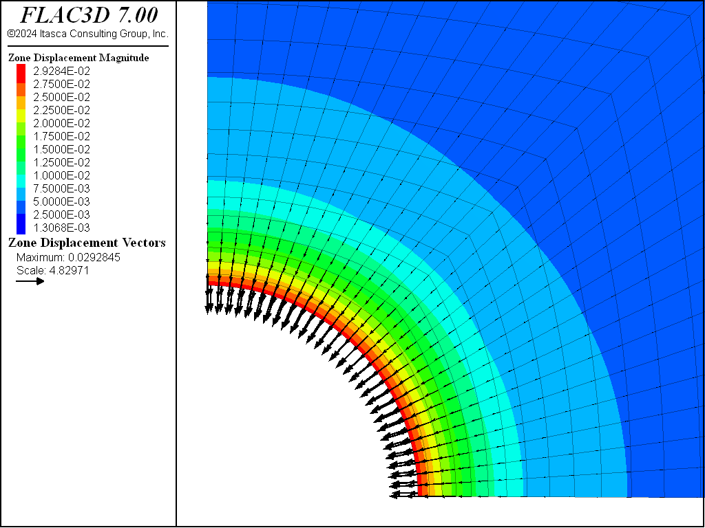
Figure 8: FLAC3D displacement contours and displacement vectors—associated.
The file “associated.dat” used to generate the associated case is shown below, “non-associated.dat” is different only in the displacement value assigned and can be found in the project. (The dilatation angle is 30° in the associated case.) The file “associated-nmd.dat” (shown below) and “non-associated-nmd.dat” generate the same two cases, but using FLAC3D’s nodal mixed discretization (NMD) feature. For the NMD models, an all-tet grid is used (“nmd.f3grid”, which is imported into FLAC3D and is generated using the “create-tet-mesh.dat” file).
The file “sale.dat” compares the numerical solutions to the analytical solution using FISH functions:
- nastr calculates (i) numerical and corresponding analytical values of \(-{\sigma}_r/P_0\) and \(-{\sigma}_{\theta}/P_0\) at the centroid of zones closest to the \(x\)-axis; and (ii) average relative error of \(-{\sigma}_r/P_0\) and \(-{\sigma}_{\theta}/P_0\) throughout the grid.
- nadis calculates (i) numerical and analytical values of \(u_r/a\) at gridpoints located on the \(x\)-axis; and (ii) the average relative error of the displacement \(u_r/a\) throughout the grid.
The resulting errors are within 2.1% of the analytical solution for stresses and displacements for both associated and nonassociated flow rules. Figure 9 through Figure 12 show the NMD results and correspond directly with Figure 4 through Figure 8 (results with an all-hex grid). As can be seen, the results are very similar.
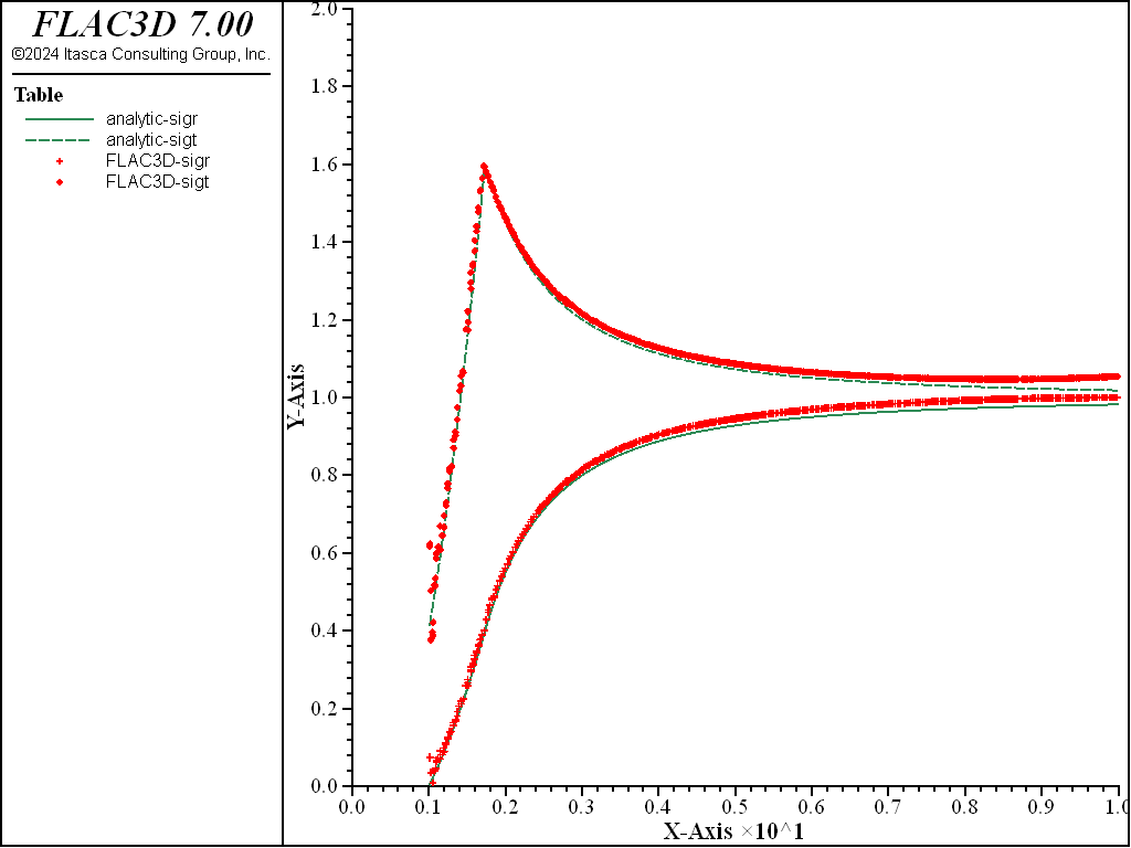
Figure 9: NMD stress solution comparison—associated (analytical values = lines; numerical values = crosses).

Figure 10: NMD stress solution comparison—nonassociated (analytical values = lines; numerical values = crosses).
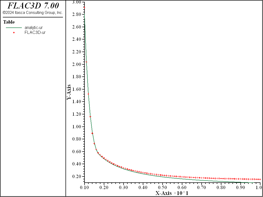
Figure 11: NMD radial displacement solution comparison—associated (analytical values = lines; numerical values = crosses).
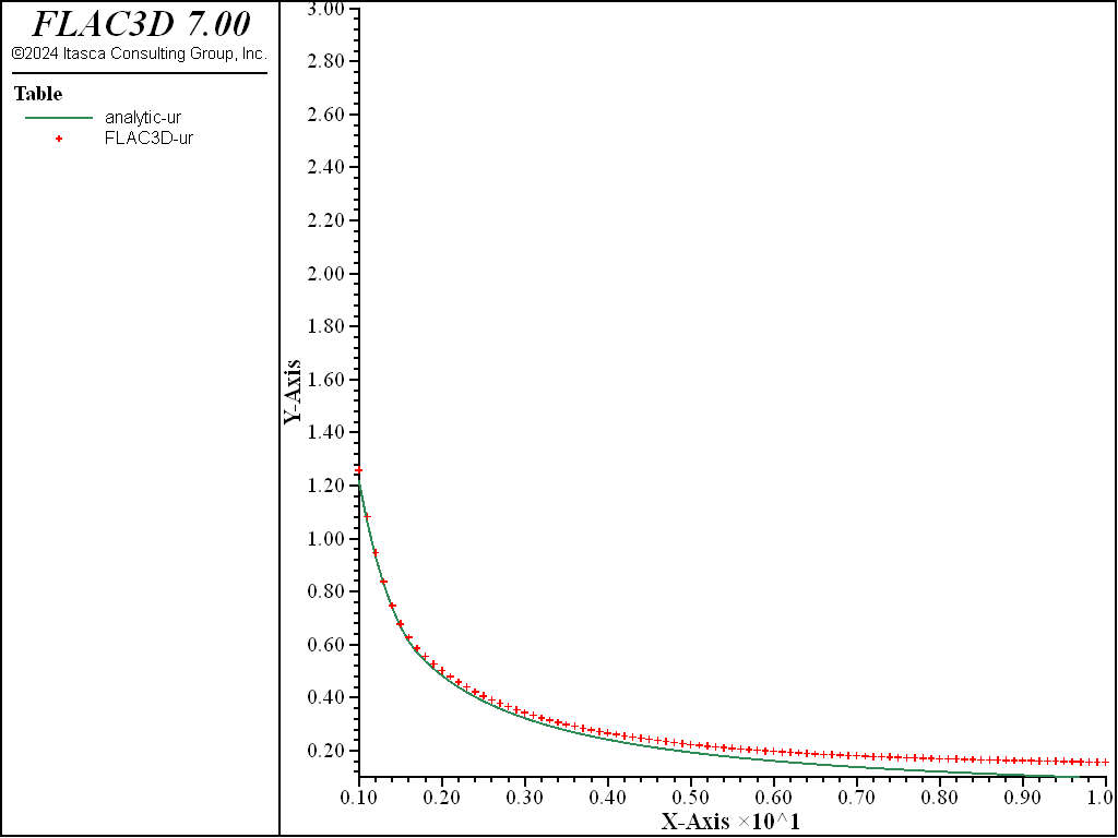
Figure 12: NMD radial displacement solution comparison—nonassociated (analytical values = lines; numerical values = crosses).
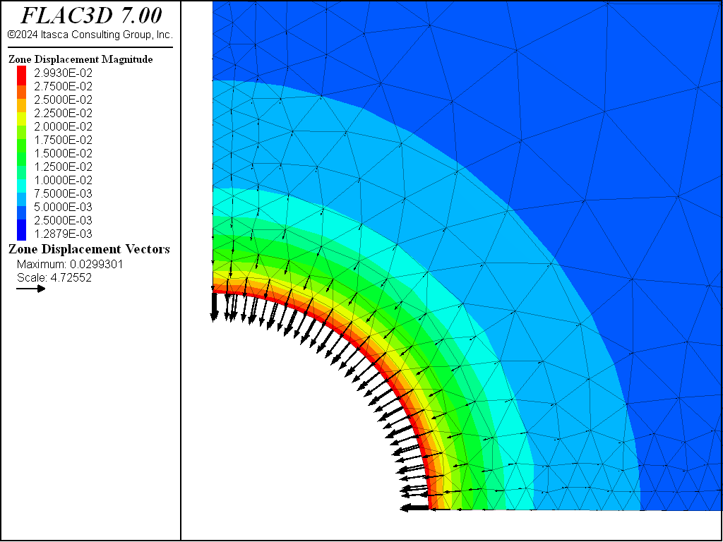
Figure 13: NMD FLAC3D displacement contours and displacement vectors—associated.
Reference
Salençon, J. “Contraction Quasi-Statique D’une Cavite a Symetrie Spherique Ou Cylindrique Dans Un Milieu Elastoplastique,” Annales Des Ponts Et Chaussees, 4, 231-236 (1969).
Data File
associated.dat
;---------------------------------------------------------------------
;            numerical solution for a long tunnel in pre-stressed
;             Mohr Coulomb material (salencon problem)
;             associated and non-associated plastic flow
;---------------------------------------------------------------------
model new
model large-strain off
; Create zones
zone create radial-cylinder size 1 1 30 30 rat 1 1 1 1.1 ...
                            point 1 10 0 0 point 2 0 0.2 0 ...
                            point 3 0 0 10 dim 1 1 1 1
; Assign constitutive model and properties
zone cmodel assign mohr-coulomb
zone property bul 3.9e9 shea 2.8e9 cohesion 3.45e6
zone property friction 30. dilation 30. tension 1.e10 ; associated flow
; Initialize stress
zone initialize stress xx -30e6 yy -30e6 zz -30e6
; Apply boundary conditions
zone face apply velocity-normal 0.0 range union position-x 0 position-z 0
zone face apply velocity-normal 0.0 range union position-y 0 position-y 0.2
zone face apply stress-normal -30e6 range union position-x 10 position-z 10
; Take some histories
model history mechanical convergence
zone history displacement-x position (1,0,0)
zone history velocity-x position (1,0,0)
history interval 1
; Solve
model solve ratio-local 1e-4
; Save the model
model save 'associated'
[io.out(string(zone.mech.ratio.local,0,' ',15))]
| Was this helpful? ... | PFC © 2021, Itasca | Updated: Feb 25, 2024 |