
Modeling Flow in Porous Media with Darcy’s Law
This example demonstrates using the Python scripting capability and the PFC CFD module to model low Reynolds number porous flow in a granular material.
Problem Description
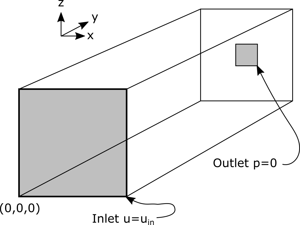
Figure 1: Schematic of problem geometry.
A granular material is contained in a rectangular box with dimensions 10 cm by 20 cm by 10 cm. Water flows into the box perpendicular to the x-z plan at y=0 at 1e-5 m3/s. The walls of the box are impermeable except for the inlet and a 2 cm by 2 cm outlet in the box on the y = 0.2 plane where the pressure is held constant. The particles making up the granular material have an average radius of 2.5e-3 m, a density of 2600 kg/m3. No gravitational forces are applied. The flow accelerates as it converges on the outlet surface. The particles are displaced through the outlet surface.
Theory
Low Reynolds number fluid flow in a porous medium is described by Darcy’s law,
where, \(\vec{v}\) is the fluid velocity, \(K\) is the matrix permeability, \(\mu\) is the fluid viscosity, \(\epsilon\) is the matrix porosity and \(p\) is the fluid pressure. It is typically assumed that the compressibility of the fluid is small enough to be neglected, leading to the incompressibility condition,
This assumption is typically taken when: (i) the fluid velocity is small compared to the sound speed of the fluid or (ii) when the expected volume change from the highest pressure to the lowest pressure in the system is small. The steady-state incompressible porous flow equation is derived by starting with (1) and taking the divergence of both sides,
substituting (2) gives,
This Poisson’s equation is subject to the following boundary conditions: \(\vec{\nabla} p= -\vec{v}_{in}\frac{\mu\epsilon}{K}\) on the inflow surface, where \(\vec{u}_{in}\) is the specified inlet velocity, \(p=0\) on the outflow surface and \(\vec{v}\cdot\vec{n}=0\) on the remainder of the boundary (where \(\vec{n}\) is the normal direction of the boundary). This equation can be solved very quickly with an implicit method to get the fluid pressure field. A single matrix inversion is required. The solution is steady state, inflow is equal to outflow. Once the pressure is known the fluid velocity can be derived from (1).
The fluid flow equations ((1) and (2)) are solved on a coarse set of elements. The fluid velocity is piece-wise linear on the elements. This set of elements (the fluid grid) is used to determined a porosity by calculating the overlap between the PFC3D particles and the fluid elements. To account for the presence of the particles on the fluid flow a permeability is calculated from the porosity of the PFC3D model. The Kozeny-Carman relation is used to estimate a permeability.
where \(r_e\) is the radius of PFC particles, and \(\epsilon_{min}\) is the minimum porosity in the system (taken as 30%). For the purpose of calculating the permeability an upper limit of porosity of 70% is taken. Above 70% porosity the permeability is taken as a fixed value.
The CFD module automatically applied the fluid-particle interaction force to the PFC particles. Two-way coupling is accomplished by updating the porosity and permeability information in the fluid-flow model and by updating the fluid-velocity field in the PFC CFD module. Short solve intervals of 100 mechanical cycles are taken in PFC punctuated by recalculating a new steady-state fluid flow field with the new porosity and permeability information. During the solve intervals in PFC the velocity field is treated as constant.
Implementation
The Python file program darcy.py implements the coupled problem.
import numpy as np
import pylab as plt
import fipy as fp
import itasca as it
from itasca import ballarray as ba
from itasca import cfdarray as ca
from itasca import element
from functools import reduce

class DarcyFlowSolution(object):
    def __init__(self):
        self.mesh = fp.Grid3D(nx=10, ny=20, nz=10,
                              dx=0.01, dy=0.01, dz=0.01)
        self.pressure = fp.CellVariable(mesh=self.mesh, \
                                        name='pressure', value=0.0)
        self.mobility = fp.CellVariable(mesh=self.mesh, \
                                        name='mobility', value=0.0)
        self.pressure.equation = (fp.DiffusionTerm(coeff=self.mobility) == 0.0)
        self.mu = 1e-3  # dynamic viscosity
        self.inlet_mask = None
        self.outlet_mask = None
        # create the FiPy grid into the PFC CFD module
        ca.create_mesh(self.mesh.vertexCoords.T,
           self.mesh._cellVertexIDs.T[:,(0,2,3,1,4,6,7,5)].astype(np.int64))
        if it.ball.count() == 0:
            self.grain_size = 5e-4
        else:
            self.grain_size = 2*ba.radius().mean()

        it.command("""
        model configure cfd
        element cfd attribute density 1e3
        element cfd attribute viscosity {}
        cfd porosity polyhedron
        cfd interval 20
        """.format(self.mu))

    def set_pressure(self, value, where):
        """Dirichlet boundary condition. value is a pressure in Pa and where
        is a mask on the element faces."""
        print ("setting pressure to {} on {} faces".format(value, where.sum()))
        self.pressure.constrain(value, where)

    def set_inflow_rate(self, flow_rate):
        """
        Set inflow rate in m^3/s.  Flow is in the positive y direction
        and is specfified on the mesh faces given by the inlet_mask.
        """
        assert self.inlet_mask.sum()
        assert self.outlet_mask.sum()
        print ("setting inflow on %i faces" % (self.inlet_mask.sum()))
        print ("setting outflow on %i faces" % (self.outlet_mask.sum()))

        self.flow_rate = flow_rate
        self.inlet_area = (self.mesh.scaledFaceAreas*self.inlet_mask).sum()
        self.outlet_area = (self.mesh.scaledFaceAreas*self.outlet_mask).sum()
        self.Uin = flow_rate/self.inlet_area
        inlet_mobility = (self.mobility.faceValue * \
                          self.inlet_mask).sum()/(self.inlet_mask.sum()+0.0)
        self.pressure.faceGrad.constrain(
            ((0,),(-self.Uin/inlet_mobility,),(0,),), self.inlet_mask)

    def solve(self):
        """Solve the pressure equation and find the velocities."""
        self.pressure.equation.solve(var=self.pressure)
        # once we have the solution we write the values into the CFD elements
        ca.set_pressure(self.pressure.value)
        ca.set_pressure_gradient(self.pressure.grad.value.T)
        self.construct_cell_centered_velocity()

    def read_porosity(self):
        """Read the porosity from the PFC cfd elements and calculate a
        permeability."""
        porosity_limit = 0.7
        B = 1.0/180.0
        phi = ca.porosity()
        phi[phi>porosity_limit] = porosity_limit
        K = B*phi**3*self.grain_size**2/(1-phi)**2
        self.mobility.setValue(K/self.mu)
        ca.set_extra(1,self.mobility.value.T)

    def test_inflow_outflow(self):
        """Test continuity."""
        a = self.mobility.faceValue*np.array([np.dot(a,b) for a,b in
                                      zip(self.mesh.faceNormals.T,
                                          self.pressure.faceGrad.value.T)])
        self.inflow = (self.inlet_mask * a * self.mesh.scaledFaceAreas).sum()
        self.outflow = (self.outlet_mask * a * self.mesh.scaledFaceAreas).sum()
        print ("Inflow: {} outflow: {} tolerance: {}".format(
            self.inflow,  self.outflow,  self.inflow +  self.outflow))
        assert abs(self.inflow +  self.outflow) < 1e-6

    def construct_cell_centered_velocity(self):
        """The FiPy solver finds the velocity (fluxes) on the element faces,
        to calculate a drag force PFC needs an estimate of the
        velocity at the element centroids. """

        assert not self.mesh.cellFaceIDs.mask
        efaces = self.mesh.cellFaceIDs.data.T
        fvel = -(self.mesh.faceNormals*\
                 self.mobility.faceValue.value*np.array([np.dot(a,b) \
                 for a,b in zip(self.mesh.faceNormals.T, \
                               self.pressure.faceGrad.value.T)])).T
        def max_mag(a,b):
            if abs(a) > abs(b): return a
            else: return b
        for i, el in enumerate(element.cfd.list()):
            xmax, ymax, zmax = fvel[efaces[i][0]][0], fvel[efaces[i][0]][1],\
                               fvel[efaces[i][0]][2]
            for face in efaces[i]:
                xv,yv,zv = fvel[face]
                xmax = max_mag(xv, xmax)
                ymax = max_mag(yv, ymax)
                zmax = max_mag(zv, zmax)
            el.set_vel((xmax, ymax, zmax))

if __name__ == '__main__':
    it.command("program call 'particles.dat'")
    solver = DarcyFlowSolution()

    fx,fy,fz = solver.mesh.faceCenters
    # set boundary conditions
    solver.inlet_mask = fy == 0
    solver.outlet_mask = reduce(np.logical_and,
                                (fy==0.2, fx<0.06, fx>0.04, fz>0.04, fz<0.06))
    solver.set_inflow_rate(1e-5)
    solver.set_pressure(0.0, solver.outlet_mask)

    solver.read_porosity()
    solver.solve()
    solver.test_inflow_outflow()
    it.command("cfd update")

    flow_solve_interval = 100
    def update_flow(*args):
        if it.cycle() % flow_solve_interval == 0:
            solver.read_porosity()
            solver.solve()
            solver.test_inflow_outflow()

    it.set_callback("update_flow",1)

    it.command("""
    model large-strain on
    model cycle 20000
    model save 'end'
    """)
The class DarcyFlowSolution uses the Finite Volume Python (FiPy)
package to solve the fluid flow equations [Guyer2009]. FiPy is part of the Python
environment which is embedded within PFC.
The file particles.p3dat creates the PFC particles and walls.
python-reset-state false
model new
model domain extent -0.01 0.11 -0.01 0.21  -0.01 0.11 condition destroy
contact cmat default model linear property kn 1e4 dp_nratio 0.2

fish define inline
  global dim = 1e-1
  global radius = dim / 10 / 4
  global xdim = dim - radius
  global ydim = 2 * dim - radius
end
[inline]

ball generate cubic box [radius] [xdim] [radius] [ydim] ...
                        [radius] [xdim] rad [radius]
wall generate box 0 [dim] 0 [2*dim] 0 [dim]
wall delete wall range id 6
wall generate polygon 0 0.2 0 ...
                      0 0.2 0.1 ...
                      0.04 0.2 0.1 ...
                      0.04 0.2 0.0

wall generate polygon 0.06 0.2 0 ...
                      0.06 0.2 0.1 ...
                      0.1 0.2 0.1 ...
                      0.1 0.2 0.0

wall generate polygon 0.04 0.2 0 ...
                      0.04 0.2 0.04 ...
                      0.06 0.2 0.04 ...
                      0.06 0.2 0.0

wall generate polygon 0.04 0.2 0.06 ...
                      0.04 0.2 0.1 ...
                      0.06 0.2 0.1 ...
                      0.06 0.2 0.06

ball attribute density 2600.0
program return
Results
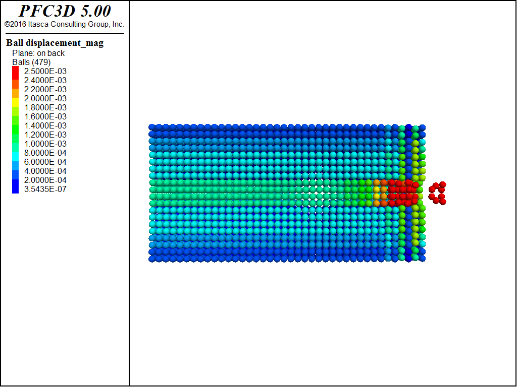
Figure 2: Color contours of particles showing displacement magnitude.
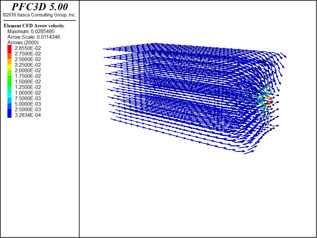
Figure 3: Fluid velocity vectors.
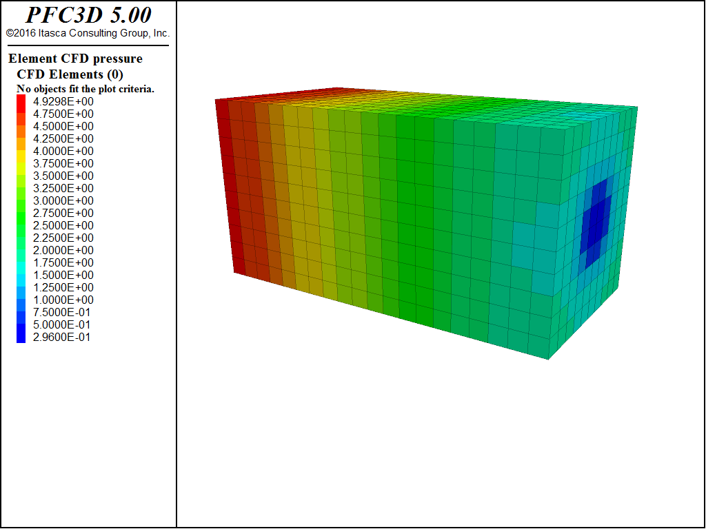
Figure 4: Fluid pressure field.
| [Guyer2009] | J.E. Guyer, D. Wheeler & J. A. Warren, “FiPy: Partial Differential Equations with Python,” Computing in Science & Engineering 11(3) pp. 6-15 (2009), doi:10.1109/MCSE.2009.52, http://www.ctcms.nist.gov/fipy |
| Was this helpful? ... | PFC © 2021, Itasca | Updated: Feb 25, 2024 |