
Faceted Walls in PFC
As discussed in “Model Components,” a PFC model is made up of bodies that interact via mechanical contacts. A faceted wall is a body composed of a triangular mesh of n facets \(\{F^{(i)}\}, i = 1, 2, ..., n\). Each facet is a piece. The \(i\)th triangular facet consists of a face bounded by three edges \(\left\{E^{(i)}_k\right\}, k=1...3\) (see Figure 1 below). The edges terminate at points, termed vertices \(\left\{V^{(i)}_k\right\}, k=1...3\). The three vertices delineating a facet must be unique. The edge vectors are defined as \(\textbf{E}^{(i)}_1 = V^{(i)}_2 - V^{(i)}_1\), \(\textbf{E}^{(i)}_2 = V^{(i)}_3 - V^{(i)}_2\), and \(\textbf{E}^{(i)}_3 = V^{(i)}_1 - V^{(i)}_3\). The vertices are ordered so that the normal, \(\textbf{n}^{(i)}\), of the facet is defined by the right-hand rule,
PFC presumes that the normals of all facets of a wall are oriented consistently with neighboring facets or those sharing a common edge or vertex (e.g., a point traversing directly above/below a faceted wall is above/below the facet closest to the traversal point except near wall boundaries). Define the signed distance from facet \(i\) to an arbitrary point in space \(P\) as \(sd = \textbf{n}^{(i)} \cdot \left(P - P^{(i)}\right)\), where \(P^{(i)}\) is any point on the plane of the facet. The distance \(sd\) is signed in the sense that \(sd > 0 \ (sd < 0)\) for points lying above (below) the facet; \(sd = 0\) for points coplanar with a facet. The wall data structure allows for the efficient identification of neighboring facets, or those sharing edges or vertices. Faceted walls can be used to represent closed or open bounded surfaces, with or without missing facets. In addition, large overlap is allowed between balls/clumps and wall facets. Note that facets are not allowed to contain internal holes; nor may facets of the same wall intersect one another. Unlike previous PFC wall implementations, walls are active on all sides by default (e.g., balls approaching facets from an inactive side do not interact with the facets). The user can flag individual facets as inactive on either or both facet sides. Note: No effort is made to stop a ball or pebble from experiencing large forces when migrating from the inactive to active side of a wall facet. Unrealistic velocities may be generated in such circumstances.
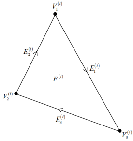
Figure 1: Depiction of a wall facet as viewed from above.
Wall motion does not obey the equations of motion. Wall motion can either be rigid or deformable, but not both simultaneously. Invoking rigid wall motion allows the user to specify a translational, \(\textbf{v}\), and a rotational, \(\textbf{w}\), velocity for the wall along with a rotational reference point, \(W_r\). Rotation is accomplished by translating all vertices so that \(W_r\) is the origin (translate by \(-W_r\)); a rotation matrix is constructed from a normalized version of the quaternion \(q(1, w_x\Delta t,w_y\Delta t, w_2\Delta t)\), where \(\Delta t\) is the timestep. The rotation matrix is applied to all vertices, which are subsequently translated by \(W_r\) to their final, rotated positions. This quaternion approach is utilized to avoid gimbal lock, which is a loss of a degree of freedom that can occur when using Euler angles. Invoking deformable wall motion allows the user to specify a translational velocity \(\left\{\textbf{v}^{(i)}\right\}, i = 1, 2, ..., m\) for each vertex in the faceted wall (\(m\) is the number of unique vertices). The specified vertex velocities must preserve facet non-intersection at all times. In all cases, the total force and moment acting on the wall (defined by \(\textbf{F}\) and \(\textbf{M}\), the sums of force and moment acting at each mechanical contact) are stored.
Mechanical interactions conceptually exist between bodies; interactions can exist between walls and bodies of other types (balls or clumps). The user does not have access to the corresponding data structures, though they are described for the sake of clarity. Inter- and intra-wall mechanical interactions are not allowed in PFC. In other words, walls do not interact with other walls. Only one mechanical interaction can exist between two different bodies, but multiple mechanical contacts may exist between the constituent pieces of those bodies. Thus a mechanical interaction acts as a container, storing a list of contacts between constituent pieces along with the resultant force and moment of all associated contacts. Mechanical interactions are created/destroyed by the contact-detection logic whenever bodies are sufficiently close/separated. Proximity detection is aided by abstracting each constituent piece of a body as an extent (e.g., an axis-aligned bounding box—as seen in Figure 2). The contact-detection scheme also creates/destroys contacts between pieces whose extents overlap. Note that there can only be one active mechanical contact between pieces—for instance, between a ball and a wall facet (including shared facet edges/vertices). As described in “Model Components,” the minimum extent can be enlarged in a user-controlled manner to ensure that interactions/contacts are created prior to the intersection of pieces of different bodies.
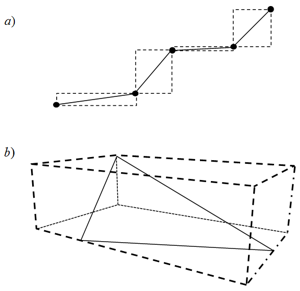
Figure 2: Minimum extents surrounding faceted walls in a) 2D and b) 3D. The black dots in a) correspond to wall edges. This document contains 2D depictions throughout.
Faceted Wall Contact Resolution
Mechanical interactions can exist between walls and balls or clumps. As both balls and clumps are composed of spherical pieces, the following discussion will focus on ball-wall mechanical interactions without loss of generality. In addition, the terms interaction and contact below refer to mechanical interactions/contacts only. An interaction is created during contact detection once a ball extent overlaps with at least one of the facet extents of a wall. This interaction holds a list of all contacts between the wall and ball. Contacts exist between the ball and each facet whose extent overlaps the ball’s extent. Contact resolution is the process by which the contact geometry and conditions are delineated. Define the wall contact point as the point on a facet with a ball-facet contact that is closest to the ball centroid (Figure 3). PFC uses an efficient algorithm that casts the triangular facets in parametric form to identify every wall contact point, including unambiguous identification of the region of the facet where the point lies (e.g., on the facet face, on one of the three edges/vertices in 3D (2 edges/vertices in 2D)). Suppose that \(l\) contacts have been identified by the contact-detection logic and that the wall contact points, \(WP_{i}, i = 1...l\), have been calculated. In addition, suppose that the contacts have been ordered with decreasing overlap. The unit normal direction of contact \(i\) points from the ball centroid \(\textbf{x}\) to the wall contact point and is given by
where \(d_i = \Vert WP_i - \textbf{x} \Vert\) is the unsigned distance from the ball centroid to the wall contact point \(WP_i\). The normal overlap between the ball and corresponding wall facet is \(U^{B,W}_i = R - d_{i}\), where \(R\) is the ball radius. The contact is active for \(U^{B,W}_i > 0\), or inactive otherwise unless the contact model stipulates different inactivity conditions. The location of the contact point, the point used for plotting and relative velocity/displacement calculations, is given by
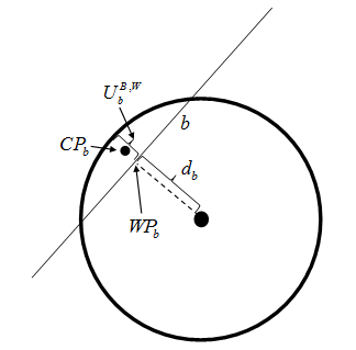
Figure 3: Definition of the overlap, \(U^{B,W}_{b}\), the wall contact point, \(WP_{b}\), and the contact point, \(CP_{b}\), for a contact with facet \(b\).
It may be undesirable in certain circumstances for multiple contacts to be simultaneously active. Suppose that a ball overlaps numerous facets delineating a flat wall (Figure 4a). Should all contacts with \(U^{B,W}_{i} > 0\) be active, the effective normal and shear contact stiffness would be many times the contact stiffness for the case of a ball overlapping a single facet (Figure 4b). Such behavior is undesirable, and an associative logic is used to determine the contact activity state. Suppose that the contacts \(C_a, C_b, C_c, C_d\) have been identified during contact detection between the ball and wall facets with corresponding wall contact points \(WP_a, WP_b, WP_c, WP_d\), respectively. All of these contacts are active (e.g., \(U^{B,W}_a, U^{B,W}_b, U^{B,W}_c, U^{B,W}_d > 0\)). Suppose that one traverses the contact list in the arbitrary order \(C_d, C_a, C_b, C_c\). Starting with contact \(C_d\), for instance, one finds that \(WP_d\) falls on the edge shared by facets \(c\) and \(d\); \(C_d\) is deemed active and a link is created between \(C_d\) and \(C_c\). This linkage between contacts occurs since a wall contact point lies on an edge shared by these two facets and \(U^{B,W}_{d} > 0\). Moving to \(C_a\), one finds that \(WP_a\) falls on the edge shared by facets \(a\) and \(b\); \(C_a\) is deemed active and a link is created to \(C_b\) as \(U^{B,W}_{a} > 0\). Moving then to \(C_b\), one finds a link to \(C_a\) and that \(WP_b\) lies on the face of facet \(b\). The linkage signifies that either \(C_a\) or \(C_b\) may be active; the condition \(U^{B,W}_{b} > U^{B,W}_{a}\) specifies that \(C_b\) is active while \(C_a\) is deemed inactive. Inspection of \(C_c\) requires a link to be created between \(C_c\) and \(C_d\) and \(U^{B,W}_{c} > U^{B,W}_{d}\), so \(C_d\) is deemed inactive. In addition, \(WP_c\) lies on the edge shared with facet \(b\) and \(U^{B,W}_{c} > 0\) so a link between \(C_c\) and \(C_b\) is created. In this case, though, \(U^{B,W}_{b} > U^{B,W}_{c}\) so \(C_c\) is also inactive. These links are depicted as curled arrows in Figure 4c. The associative contact-resolution strategy for ball-facet contacts produces the desired result of one active contact, namely \(C_b\). The rules for this scheme can be summarized as follows: 1) only one active contact can exist between a ball and a wall facet, including shared edges and vertices; 2) contacts between a ball and adjacent facets with wall contact points on a shared edge or vertex are linked, provided that the normal overlap is greater than 0; and 3) the contact with the largest overlap in a linked set is the only active contact.
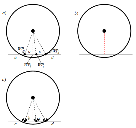
Figure 4: From top left: a) Ball overlapping coplanar wall segments with the wall contact points delineated by the intersections of the dashed lines and the wall facets. b) Ball overlapping a single wall facet. The red dashed line is the active contact. c) Same as a), except the links between contacts are shown as curled, double arrows and the red dashed line corresponds to the active contact with facet \(b\).
The application of this algorithm to a ball traversing a wall toward a convex edge is depicted in Figure 5. The wall has been broken into multiple facets to demonstrate the use of the algorithm. Figure 5a shows that the contact with facet \(c\), \(C_c\), is active and linked to \(C_b\) and \(C_d\), which are inactive. In addition, \(C_a\) is inactive and linked to \(C_b\). In Figure 5b, \(C_c\) remains active and linked to the inactive contacts \(C_d\) and \(C_b\). The gray region is the region where the ball transitions over the edge shared with facets \(c\) and \(d\). As this happens (Figure 5b and Figure 5c), the contact normal smoothly rotates and \(C_c\) continues to be active. Once over the shared edge (Figure 5d), \(C_d\) becomes active and is linked to the inactive \(C_c\) and \(C_e\). \(C_e\) is also linked to \(C_f\), which is inactive.
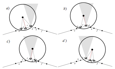
Figure 5: From top left: a) Ball approaching a convex facet edge. Links are depicted by curled, double arrows. The gray region corresponds to the region directly above the edge. The active wall contact point lies at the end of the red dashed line. The black dashed lines terminate at inactive wall contact points. b) The active wall contact point falls on shared edge between facets \(c\) and \(d\). c) The contact normal naturally migrates through the region above the edge. d) Contact activity passes the region above the edge.
The algorithmic performance when applied to a ball moving toward a concave edge is demonstrated in Figure 6. Figure 6a depicts the situation where the ball has not yet begun to overlap the opposing wall facets. In Figure 6b, the algorithm results in two active contacts, namely \(C_c\) and \(C_d\). This occurs because these contacts are not linked, because a wall contact point does not lie on a shared edge or vertex. As the ball continues to translate, \(C_e\) is the only active contact (Figure 6c). When applied to a case of a nominally flat wall with roughness at a length scale much less than the ball size (as seen in Figure 7), this algorithm results in active contacts at each of the facet edges/vertices closest to the ball centroid. This wall configuration results in a significantly stiffer ball-wall contact interaction, because the ball is interacting with a number of facet edges. Though this wall segment is flat when viewed at a certain scale, it does not behave as the examples shown in Figure 4, given application of the associative algorithm. The application of the associative logic is facilitated by ordering the contacts with decreasing overlap; associative checks cease once these checks have been applied to all contacts with positive overlap. The associative logic, as outlined, is included in both “reduced” and “full” contact resolution modes.
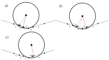
Figure 6: From top left: a) Ball approaching a concave facet edge. See the previous figure for a description of the line conventions. b) The wall contact points of the two active contacts (termination of red dashed lines) fall on either side of the concave edge. c) One active contact remains.
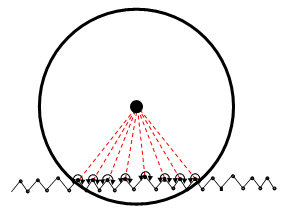
Figure 7: Ball overlapping a nominally flat wall with roughness smaller than the ball size.
Two circumstances where the associative logic will not produce the desired behavior are shown in Figure 8. In Figure 8a, a ball overlaps a sliver where no link exists between contacts. In Figure 8b, a ball overlaps multiple facets of the same wall and no links are present. These situations can occur when the scale of a feature of a wall is much smaller than the scale of a ball. Application of the associative logic results in two (three) active contacts in Figure 8a (Figure 8b) where only one active contact may be physical in both cases. Such conditions can be detected by determining whether or not the line segments connecting the ball centroid to the wall contact points of active contacts (active as determined by the associative logic) intersect any other facets with active contacts. The contact with the largest overlap is deemed active. Such a check is unnecessary when the scales are compatible and is not included in “reduced” contact resolution mode (the default behavior). An alternate approach to mitigating the wedge situation in Figure 8a is to set the “inner” facets of the wedge as inactive, resulting in only one active contact. Such a solution would not mitigate the situation in Figure 8b, though. It is advisable that one consider setting the scales of wall features and balls to be similar, to avoid these situations.
Figure 8: Situations where the associative logic fails. a) Ball intersecting a thin wedge and b) ball intersecting multiple segments. The “full” contact resolution mode includes the check for this condition, while the “reduced” mode does not.
Continuity of Contact-State Information
Suppose that one uses the default contact model in PFC with nonzero normal/shear stiffness and a very large friction coefficient to simulate the two examples shown in Figure 4a and Figure 4b. As the ball translates a specified distance over numerous timesteps along the single facet (Figure 4b), the shear force incrementally accumulates. As the active contact transitions from one facet to another in the multi-facet example (Figure 4a), one is faced with the problem of enforcing continuity in contact-state information in order for the two examples to yield identical results. No continuity in contact-state information, for instance, will lead to the loss of shear force in this situation as the ball moves. Contact-state information is only propagated when in “full” resolution mode. Suppose that the contact-state information is retained during one contact-resolution session when a contact state is switched from active to inactive (e.g., contact normal, wall contact point, contact point, force, moment, etc.). Take the configuration shown in Figure 9a and Figure 9b to correspond with the model state at time \(t\) (\(t + 1\) or incremented by one timestep). \(C_b\) is active at time \(t\), and \(C_d\) is active at time \(t + 1\). Suppose also that the wall facet normals are given by \(\textbf{n}_b\) and \(\textbf{n}_d\) for facets \(b\) and \(d\), respectively. The angle between these facet normal vectors is given by \(\theta = \arccos(\textbf{n}_b \cdot \textbf{n}_d)\). Let the user define the cutoff angle \(\Theta \geq 0\) for all wall interactions with a specific wall. Should \(\theta \leq \Theta\) and no holes exist between the two facets in question, the non-geometric contact-state information is propagated (e.g., all information but not the normal, wall contact point, contact point, etc.). Each contact model defines the process by which the contact-state information is propagated, and this state information can only be propagated between contacts utilizing the same contact models. For the linearbond contact model, the forces are moments added to the currently stored values. The term hole is used to define two conditions: 1) a continuous path cannot be constructed via facet adjacency information between two facets where each facet along the path must intersect the plane containing the wall contact points at subsequent timesteps, \(WP_b\) and \(WP_d\), with normal perpendicular to the average contact normal; or 2) the angle between \(\textbf{n}_b\) and one of the facets along the path is greater than \(\Theta\). In this example, \(\theta = 0\) and a continuous path can be constructed from facets \(b \rightarrow c \rightarrow d\) with no holes; thus the contact-state information is copied from \(S_b\) to \(S_d\).
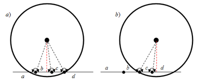
Figure 9: From left: a) shows wall traversing coplanar facets as in Figure 4a at time \(t\); b) shows configuration at time \(t + 1\).
The associative logic is used as a proxy for path construction. If no links exist between a previously active contact and a contact that has been deemed active by the contact resolution scheme, then the contact-state information is not propagated. For instance, the cases shown in the next figure are easily handled without any direct path construction, due to the associative logic.
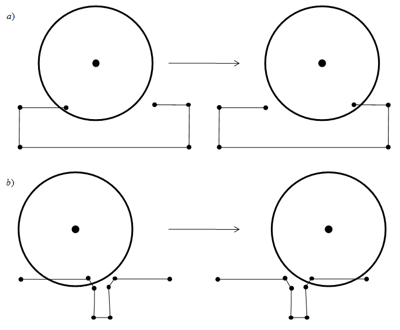
Figure 10: Two cases demonstrating the need for hole checking. Configurations on either side of the arrows are one timestep apart.
Continuity of Contact-State Information at Concave Edges – Proximity Contacts
Suppose that a ball approaches a concave edge as shown in Figure 6a. Take these snapshots as subsequent timesteps of a simulation. Application of the algorithm described in the previous section results in the contact-state information being copied from \(C_b\) to \(C_c\) for the configuration in Figure 6b. Assume that \(\arccos(\textbf{n}_b \cdot \textbf{n}_d), \arccos(\textbf{n}_c \cdot \textbf{n}_d) \leq \Theta\). There is no propagation of state information to \(C_d\). In Figure 6c, \(C_c\) has become inactive and the associated contact-state information has been lost, given the rules outlined above. In order to accommodate the need for continuity of state information across concave facet edges, the algorithm is augmented by the following rule: any two active contacts where the angle between facet normals is less than \(\Theta\) (\(C_d\) and \(C_d\) in Figure 6b) are combined into a single, active proximity contact. Only the proximity contact (PC) accumulates force/moment. The PC has a normal equal to the overlap weighted normal, for example,
with overlap equal to the average overlap. Once a proximity contact has been created, contacts with facets adjacent to those included in the proximity contact are checked for inclusion in the proximity contact. Thus contacts with facets adjacent to those included in a proximity contact where 1) there is a positive overlap and 2) where the minimum angle between any facet normal of facets in the proximity contact are added to a proximity contact. Once a contact overlap is negative, the contact is removed from the proximity contact.
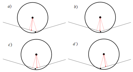
Figure 11: Configurations of a ball traversing a concave facet edge. The dashed red lines end at the wall contact points of the active contacts without application of the PC logic. The solid red lines terminate at the PC wall contact points when this logic is applied.
The PC logic also has an impact on the resulting contact configuration of the example presented in Figure 7. Application of the algorithm will reduce the number of active contacts considerably, depending on the value of \(\Theta\) assigned by the user.
| Was this helpful? ... | PFC © 2021, Itasca | Updated: Feb 25, 2024 |