
ball distribute command
Syntax
- ball distribute keyword ... <range>
Primary keywords:
Distribute balls with overlaps. This process ceases when a target porosity (not accounting for overlap) is achieved. By default, the ball positions and radii are drawn from uniform distributions throughout the model domain. As a result, the set of balls generated is affected by the state of the random-number generator (see
model random). The ball radii can also be drawn from a Gaussian distribution via the gauss keyword. A number of ball distributions, with radius ranges and volume fractions, can be specified. The optional range is applied to each ball upon generation, ensuring that the final distribution meets the target criteria. This command contrasts with theball generatecommand where balls, with radii chosen from a single distribution, are generated without overlap until either 1) the target number of balls is met or 2) the number of attempts to place balls meets the defined criteria.Note
- A model domain must be specified prior to ball generation.
- Significant ball overlaps will likely result from this operation.
- While cycling, balls can only be created before cycle point 0 (i.e., when the timestep is calculated).
- bin i keyword ...
Specify the distributional properties of bin i. Any number of distributions with radii ranges, volume fractions, and distributional types can be specified. The volume fractions of all distributions must sum to 1.
- fish-distribution s a1...an
The ball radii are drawn from the distribution represented by the FISH function s. Function arguments can be specified as though no function arguments are required. The FISH function must return a floating point value that is the ball radius. A FISH distribution cannot be specified with the gauss or radius keywords.
- gauss <f >
Specify that the ball radii are chosen from a Gaussian distribution with mean value (fradlow + fradhi)/2 and standard deviation (fradhi - fradlow)/2. The optional f (default 0.1), multiplied by fradlow, constitutes the minimum radius allowed.
- group s <slot slot > ...
Specify that generated balls are given group name s at slot slot. If the slot keyword is not specified, then the group name is assigned to the slot Default.
- radius fradlow <fradhi >
Specify the radius range to be used during generation. If fradhi is not specified, then fradhi = fradlow. By default fradhi = fradlow = 1.0. Cannot be given with the fish-distribution keyword.
- volume-fraction f
The volume fraction of balls in this distribution. The sum of volume fractions of all distributions must be 1.
- box fxmin fxmax <fymin fymax <fzmin fzmax >> (`z`-components are 3D ONLY)
Ball will fully fall within this box, such that they will not overlap the box faces or edges. If the y,z-boundaries are omitted, they will be taken as equal to the \(x\)-boundaries. If the \(z\)-boundaries are omitted, they will be taken equal to the \(y\)-boundaries. By default, the box is the model domain.
- number-bins i
Number of distributions used to generate the assembly.
Usage Example
The ball distribute command is one of the three commands that can be used to create balls. Alternative commands
are ball generate and ball create. As discussed in the command description above, ball distribute will distribute
balls within a given range to achieve a target porosity, but will not check for overlapping balls during this process.
Simple example
The following code distributes balls with radii ranging from 1.0 to 1.6 in the entire domain
extent, with a target porosity of 0.36. The system is shown in Figure 1. Note that because the
ball distribute command does not check for overlaps when positioning the balls, large overlaps exist in the model at this stage.
; setup model domain and CMAT
model domain extent -25.0 25.0 condition periodic
contact cmat default model linear method deformability emod 1e6 ...
                                         kratio 1.25 property fric 0.25
; generate balls
ball distribute radius 1.0 1.6 porosity 0.30
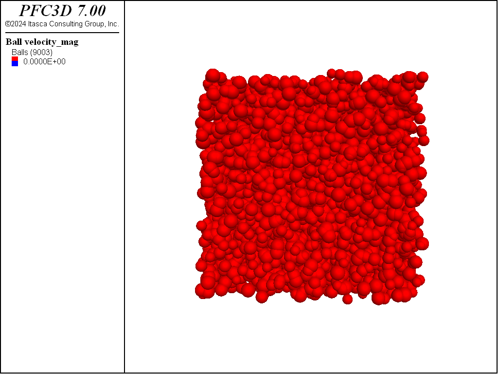
Figure 1: Specimen after execution of the ball distribute command. Note that large overlaps
exist between balls.
After the command is executed, overlaps may be reduced by letting the balls rearrange. The code below
will perform this operation by solving the system to the default target criterion. Note that the model cycle command
is initially issued along with the calm keyword to efficiently remove energy from the system. The final
system is shown in Figure 2.
model large-strain on
ball attribute density 1000.0 damp 0.7
model cycle 1000 calm 100
model solve

Figure 2: Specimen after a solve sequence. Balls have rearranged to minimize overlaps.
It is worth noting that the ball distribute command is self contained, meaning that the result
of its execution does not account for any balls that may already exist in the model. For instance,
if the command is executed one more time with the following line, then the final state will contain both the balls
previously created and newly created balls, as shown in Figure 3.
ball distribute radius 1.0 1.6 porosity 0.30
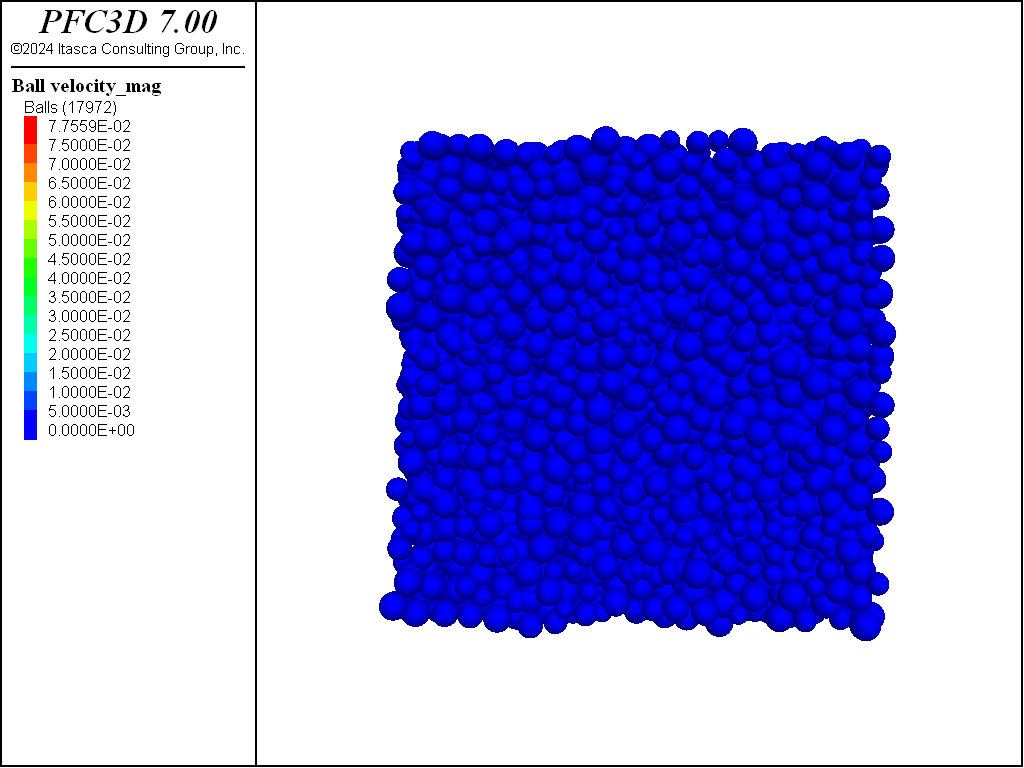
Figure 3: System after another execution of the ball distribute command. Note that balls have
been created although the specimen target porosity was already met. The command is self contained and
does not account for pre-existing balls in the model.
Bimodal particle-size distribution
The following example produces a bimodal assembly of balls comprised of 25% small balls
(with radii ranging from
0.2 to 0.32) and 75% large balls (with radii ranging from 0.4 to 0.6). Note the use of the
resolution keyword, along with a value of 0.2, which is used to
multiply the specified radii. The balls are generated within a spherical range
(obtained through a geometry object, which is also used to create a corresponding wall)
with a target porosity of 0.36.
Density and local damping attributes are specified and the system is solved using timestep
scaling (see the model mechanical timestep command).
The final distribution is shown in Figure 4.
model new
model large-strain on
; define the domain extent and the default slots of the CMAT
model domain extent -10 10
contact cmat default model linear method deformability emod 1e6 ...
                                         kratio 1.25 property fric 0.25

; generate a sphere geometry and import it as a wall
geometry set 'sphere'
geometry generate sphere radius 5.0
wall import from-geometry 'sphere'

; use the ball distribute command to create a bimodal assembly
; use the sphere gemoetry as a filtering range
ball distribute porosity 0.36                 ...
                resolution 0.2                ...
                number-bins 2                     ...
                bin 1                         ...
                  radius 1.0 1.6              ...
                  volume-fraction 0.25         ...
                  group 'small'               ...
                bin 2                         ...
                  radius 2.0 3.0              ...
                  volume-fraction 0.75         ...
                  group 'large'               ...
                range geometry-space 'sphere' count 1

; set ball desnity and local damping coefficient
; and solve the system
ball attribute density 1000.0 damp 0.7
model cycle 1000 calm 100
ball delete range geometry-space 'sphere' count 1 not
model mechanical timestep scale
model solve ratio-average 1e-3
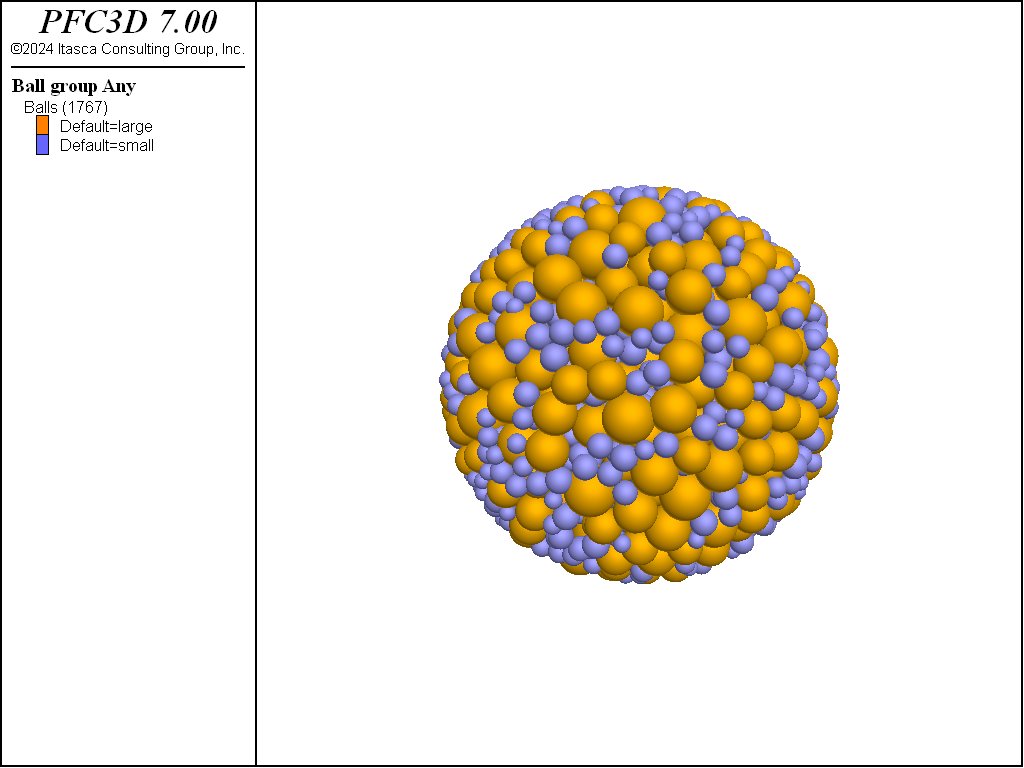
Figure 4: Final bimodal assembly (balls colored by group name).
Any number of bins can be specified to match a real particle-size distribution measured experimentally. The tutorial example “Replicating a Particle Size Distribution” illustrates how this can be achieved.
| Was this helpful? ... | PFC © 2021, Itasca | Updated: Feb 25, 2024 |