Elastic Plate (Infinite Strip) with Uniform Lateral Load

Problem Statement

Note

To view this project in FLAC3D, use the menu command Help ► Examples…. Choose “Structure/Shell/InfiniteStrip” and select “InfiniteStrip.prj” to load. The main data file is shown at the end of this example.

The displacement field, bending and transverse-shear stress resultants for a rectangular elastic plate simply supported along two edges and subjected to a uniform lateral load are computed and compared with the analytical solution for an infinite strip. This problem quantifies the ability of the DKT shell element to model the bending action.

Analytical Solution

A plate in the form of an infinite strip that is simply supported along two edges is subjected to a uniform lateral load. The plate has an isotropic elastic material model. The analytical solution for lateral deflection as well as bending and transverse-shear stress resultants is given by Ugural (1981, Example 1.1). The load is resisted by bending action, and thus, the membrane stress resultants are zero. The analytical solution is for the infinite strip shown in Figure 1.

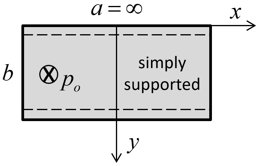
Figure 1: Infinite strip, lateral loading and coordinate system used to express the analytical solution.

The lateral deflection is given by

\[w = {p_o b^4 \over 24D} \left( {y^4 \over b^4 } - 2{y^3 \over b^3} + {y \over b} \right),\quad D = {Et^3 \over 12(1-\nu^2)}\]

where \(p_o\) is applied pressure; \(b\) is strip width; \(D\) is flexural rigidity; \(E\) is Young’s modulus; \(\nu\) is Poisson’s ratio; and \(t\) is strip thickness.

The bending stress resultants are

\[M_x = -\nu D{d^2 w \over dy^2 },\quad M_y = -D{d^2 w \over dy^2 },\quad M_{xy} = 0\]

which can be expressed as

\[M_x = -\nu M_y,\quad M_y = {-p_ob \over 2} \left( {y^2 \over b} - y \right),\quad M_{xy} = 0\]

The transverse-shear stress resultant is

\[Q_x = {\partial M_{xy} \over \partial y} + {\partial M_x \over \partial x},\quad Q_y = {\partial M_{xy} \over \partial x} + {\partial M_y \over \partial y}\]

which can be expressed as

\[Q_x = 0,\quad Q_y = {-p_o b \over 2 } \left( {2y \over b} - 1 \right)\]

FLAC3D Model

The infinite strip is modeled as a finite-sized rectangular plate of length \((a)\) and width \((b)\) using a 16 by 8 mesh of DKT elements with a cross-diagonal pattern as shown in Figure 2. The cross-diagonal pattern is used to ensure symmetric response. The simply-supported boundary condition (translational velocity fixed in the \(z\) direction) is assigned to the nodes along the \(y=0\) and \(y=b\) lines. Rigid-body motion is prevented by fixing the \(x\) and \(y\) translational of the upper-left node, and fixing the \(y\) translation of the lower-right node. The uniform lateral load is applied over the plate surface as a uniform pressure acting in the positive \(z\) direction. The \(z\)-displacement at the plate center is monitored as a history. Local nonviscous damping is used with a damping factor of 0.8. The model is run in small-strain mode to correspond with the small-strain assumption of the analytical solution. The model is cycled until a convergence limit of \(1 \times 10^{-3}\) is achieved. The model response is compared with the analytical solution along the \(x=0\) line, where the response of the finite-sized plate is like that of the infinite strip.

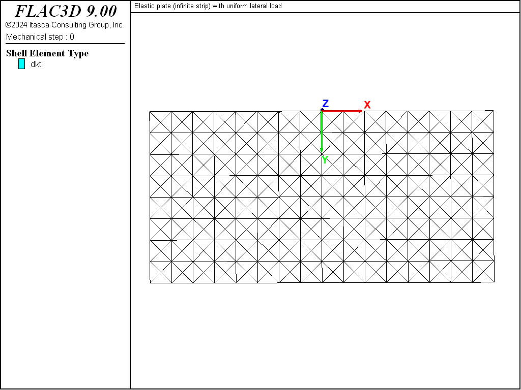
Figure 2: Geometry of the FLAC3D model showing mesh and global coordinate system.

The particular properties used for this problem are defined as follows. Consider a 4 by 8 sheet of three-quarter inch plywood that spans a trench of width \((b)\) and is simply supported along its long edges:

\[\begin{split}\begin{gather} t = 19 \textrm{ mm}, \quad a = 2440 \textrm{ mm}, \quad b = 1220 \textrm{ mm} \\ \bigl[ \textrm{thin plate: }b/t > 20, \quad \textrm{infinite strip: }a>>b \bigr] \end{gather}\end{split}\]

The plywood is assumed to behave as an isotropic elastic material:

\[E = 8.5 \textrm{ GPa}, \quad \nu = 0.33\]

A box of dry sand that is one-half meter deep sits on top of the plywood sheet, inducing a uniform lateral load:

\[\begin{split}\begin{gather} p_o = \rho g H = 7.86 \textrm{ kPa} \\ \bigl[ \rho = 1602 \textrm{ kg} / \textrm{m}^3,\ g = 9.81 \textrm{ m} / \textrm{s}^2,\ H = 0.5 \textrm{ m} \bigr] \end{gather}\end{split}\]

Results and Discussion

The deformed shape and center-deflection history are shown in Figure 3, from which we conclude that the static solution has been obtained. The lateral deflection along the \(x=0\) line is compared with the analytical solution in Figure 4. The lateral deflection is obtained from the \(z\) displacement of the nodes along the \(x=0\) line. The computed deflection is within 1.5% of the analytical values at all sampling locations.

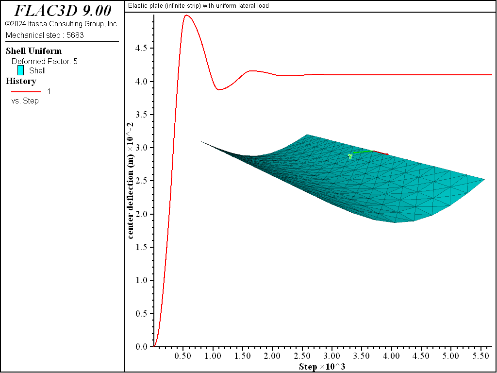
Figure 3: Deformed shape (deformation factor: 5) and center deflection.

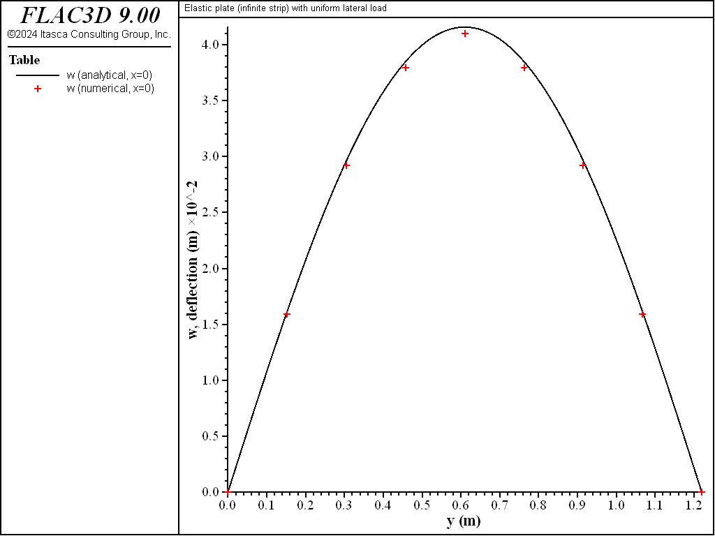
Figure 4: Lateral deflection along the \(x=0\) line.

The stress resultants are expressed in a surface coordinate system that is aligned with the global coordinate system. The stress resultant field variations are displayed as contours using the Structural Element:Shell plot item, and checking the Use Engine Data box (discussed here).

The bending along the strip length is quantified by the \(M_y\) stress resultant and shown in Figure 5. The field is constant along the length and varies from near-zero at the ends to maximum at the centerline. \(M_y\) along the \(x=0\) line is compared with the analytical solution in Figure 6. The values of \(M_y\) are obtained at the nodes along the \(x=0\) line. These values have been averaged for the shell elements that share each node. The computed values are within 0.9% of the analytical values at all sampling locations where the analytical values are not zero. The values at the ends are not zero, but will approach zero as the mesh is refined.

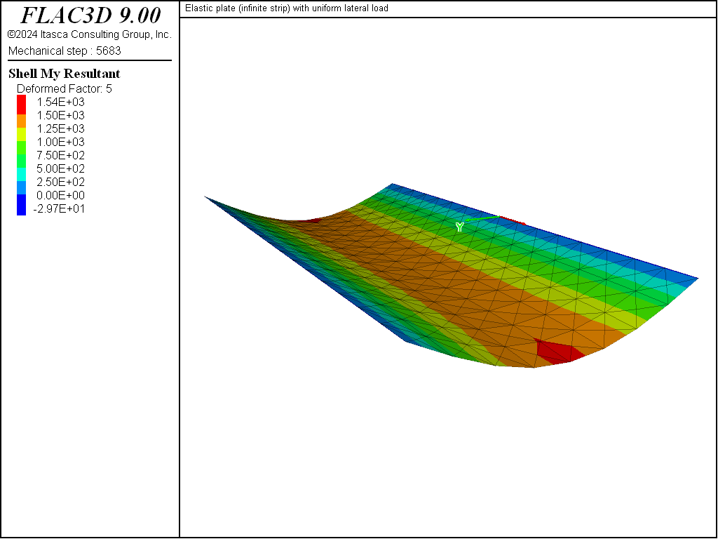
Figure 5: \(M_y\) stress resultant plotted on deformed shape (deformation factor: 5).

Figure 6: \(M_y\) stress resultant along the \(x=0\) line.

The variation of the \(M_x\) stress resultant over the strip surface is shown in Figure 7. \(M_x\) along the \(x=0\) line is compared with the analytical solution in Figure 8. The values of \(M_x\) are obtained at the nodes along the \(x=0\) line. These values have been averaged for the shell elements that share each node. The computed values are within 2.4% of the analytical values at all sampling locations where the analytical values are not zero. The values at the ends are not zero, but will approach zero as the mesh is refined.

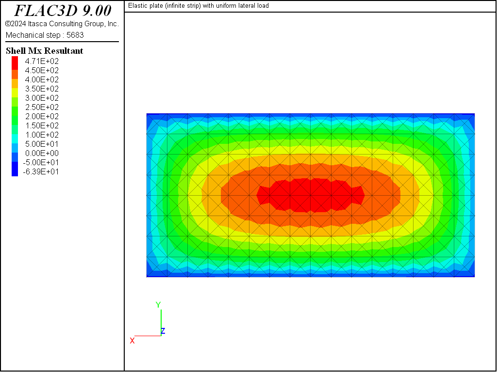
Figure 7: Variation of the \(M_x\) stress resultant over the strip surface.

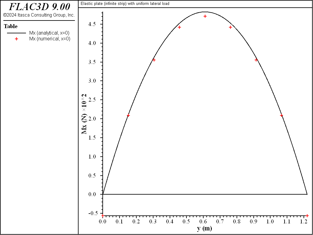
Figure 8: \(M_x\) stress resultant along the \(x = 0\) line.

The variation of the \(Q_y\) stress resultant over the strip surface is shown in Figure 9. \(Q_y\) along the \(x=0\) line is compared with the analytical solution in Figure 10. The values of \(Q_y\) are obtained at the centroids of the shell elements just to the side of the \(x=0\) line — there is no averaging at nodes. The computed values are within 4.1% of the analytical values at all sampling locations. The transverse-shear stress resultants are computed with less accuracy than the bending stress resultants because the transverse-shear stress resultants are obtained from the spatial derivatives of the bending stress resultants (shown here) — taking spatial derivatives reduces accuracy.

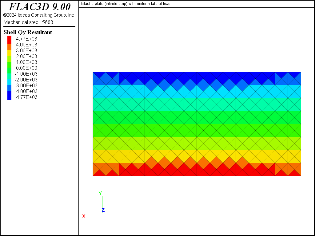
Figure 9: Variation of the \(Q_y\) stress resultant over the strip surface.

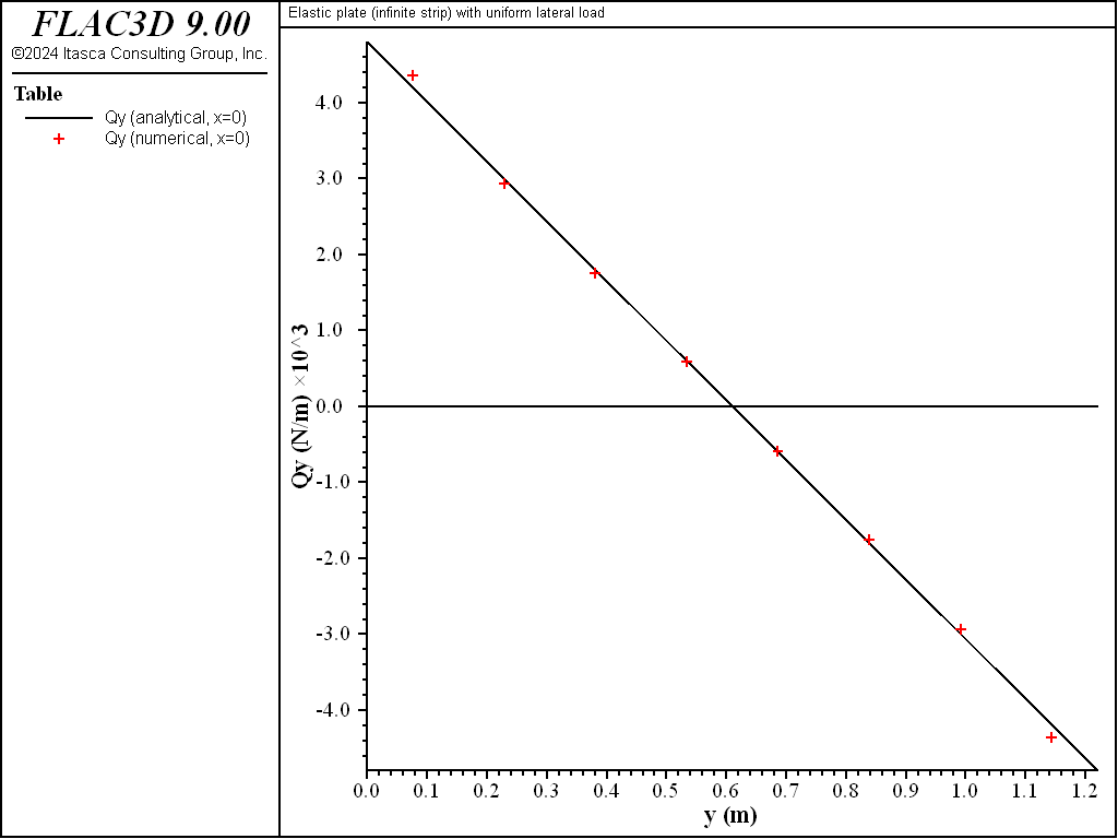
Figure 10: \(Q_y\) stress resultant along the \(x = 0\) line.

Reference

Ugural, A. C. Stresses in Plates and Shells, New York: McGraw-Hill Publishing Company, Inc. (1981).

Data File

InfiniteStrip.dat

model new
fish automatic-create off
model title 'Elastic plate (infinite strip) with uniform lateral load'
; =============================================================================
; Material properties and dimensions (SI units)
  [global E  = 8.5e9]  ; plywood
  [global nu = 0.33]
  [global t =   19e-3]  ; ~ 3/4 inch
  [global a = 2440e-3]
  [global b = 1220e-3]
  [global rho = 1602]  ; dry sand
  [global Ht = 500e-3] ; height of sand
; Derived items
  [global p0 = rho * 9.81 * Ht] ; units: N/m*m
  [global D = E*t*t*t/(12 * (1 - nu*nu))
; Properties of mesh
  [global crossDiag = true]
  [global nx = 16]  ; should be even
  [global ny =  8]  ; should be even
; =============================================================================
; Create mesh, assign shell properties, apply boundary conditions.
structure shell create by-quadrilateral ...
             ([-0.5*a],0,0) ([0.5*a],0,0) ([0.5*a],[b],0) ([-0.5*a],[b],0) ...
             size [nx] [ny]  cross-diagonal  [crossDiag] element-type dkt
structure shell property thickness [t]
structure shell cmodel assign elastic
structure shell property young [E] poisson [nu]

structure node group 'top'    slot 'BCs' range position-y 0.0
structure node group 'bottom' slot 'BCs' range position-y [b]
; BCs: simply supported sides, fixXY in upper left, fix y in lower right
structure node fix velocity-z range group 'top' group 'bottom' union
structure node fix velocity-x velocity-y ...
                range component-id [struct.node.id(struct.node.near(-0.5*a, 0, 0))]
structure node fix velocity-y ...
                range component-id [struct.node.id(struct.node.near( 0.5*a, b, 0))]
structure shell apply [p0]

structure node history displacement-z position 0.0 [0.5*b] 0  ; plate center

model large-strain false
structure mechanical damping local 0.8
model save 'initial'
model solve convergence 1e-3

structure shell recover surface 1 0 0 ; align with the global x and y direcs.
structure shell recover resultants

model save 'final'