Stress Boundary
By default, the boundaries of a 3DEC model are free of stress and any constraint. Forces or stresses may be applied to any boundary, or part of a boundary, with the block face apply command. Note that forces and stresses can be applied to either rigid or deformable blocks. Individual components of the stress tensor (\(\sigma_{xx}\), \(\sigma_{yy}\), \(\sigma_{zz}\), \(\sigma_{xy}\), \(\sigma_{xz}\) and \(\sigma_{yz}\)) are specified with the stress keyword. For example, the command
block face apply stress 0,0,-1e6 0,0,0 range pos-x 0 10 pos-y -1 1 pos-z 0 10
would apply \(\sigma_{xx}\) = 0, \(\sigma_{yy}\) = 0, \(\sigma_{zz}\) = −10:sup:6 and zero shear stresses to a model boundary lying within the coordinate window 0 < \(x\) < 10, −1 < \(y\) < −1, 0 < \(z\) < 10. The user should always make sure that the window encompasses all of the boundary vertices designated for the assigned boundary condition. This can be done using the Boundary Conditions plot item.
It is also possible to apply individual stress components. For example:
block face apply stress-zz -1e6 range pos-z 10
Compressive stresses have a negative sign, in accordance with the general sign convention for internal stresses in 3DEC. Also, 3DEC actually applies stress components as forces, or tractions, which result from a stress tensor acting on the given boundary plane. The tractions are divided into two components, permanent and transient. Permanent tractions are constant loads, and transient tractions are time-varying loads applied for dynamic analysis (see Application of Dynamic Input) by using the fish or table keyword on the same command line as the stress keyword.
Individual forces can be applied to the model boundary of rigid or deformable blocks by using the block gridpoint apply command with the force-x, force-y, or force-z keywords, which specify \(x\)-, \(y\)- and \(z\)-components of an applied force vector. Note that forces are applied to gridpoints and stresses are applied to faces.
Applied Stress Gradient
The block face apply command may take additional keywords gradient-x, gradient-y, and/or gradient-z which allow the applied stresses to vary linearly over the specified range. Six parameters follow each of these keywords and describe the variation of the stress components in the \(x\)-, \(y\)- or \(z\)-direction:
gradient-x sxxx syyx szzx sxyx sxzx syzx
gradient-x sxxy syyy szzy sxyy sxzy syzy
gradient-x sxxz syyz szzz sxyz sxzz syzz
The stresses vary linearly with distance from the global coordinate origin of \(x\) = 0, \(y\) = 0, \(z\) = 0:
where \(\sigma^\circ_{xx}\), \(\sigma^\circ_{yy}\), \(\sigma^\circ_{zz}\), \(\sigma^\circ_{xy}\), \(\sigma^\circ_{xz}\), and \(\sigma^\circ_{yz}\) are the stress components at the origin.
The operation of this feature is best explained by an example:
block face apply stress 0,0,-10e6 0,0,0 grad-z 0,0,1e5 0,0,0
The stresses at the origin (\(x\) = 0, \(y\) = 0, \(z\) = 0) are:
The equation for the \(z\)-variation in stress component \(σ_{zz}\) is
The value for \(\sigma_{zz}\) at \(z\) = −100 is then −20 × 106. At points in between, the \(z\)-variation is linearly scaled to the relative \(z\)-distance from the origin.
It is also possible to apply a gradient to a single stress component. In this case, the input is a vector giving the variation of that component in the \(x\), \(y\) and \(z\) directions. The following example would produce the same result as the example above:
block face apply stress-zz gradient 0 0 10e5
Typically, applied stress gradients are used to reproduce the effects of increasing stress with depth caused by gravity. It is important to make sure that the applied gradient is compatible with the gradient specified with the :cmd:block.insitu` command and the value of gravitational acceleration (model gravity command).
Changing Boundary Stresses
As discussed above, transient loading can be performed with the fish or table keyword for dynamic analysis. For static analysis, it may also be necessary to alter the values of applied stresses during the course of a 3DEC simulation. For example, the load on a footing may change. To effect a sudden change in an existing applied stress or load, a new block face apply command is given with the range that encompasses the same boundary vertices as in the original command, but with a change in stress value or variation.
Note
*The user should be aware that this approach is different than the one used in the Itasca code FLAC, in which the stresses are updated to the new values when a new boundary condition is specified.
In this case, the new value will be added to the existing value.* If the stress is to be removed, the current value should be given with an opposite sign. If a transient load is changed (i.e., a load assigned with the fish or table keyword), any new load with the same history type is added to the existing load; however, a new transient load with a different history type replaces the old transient load.
Checking the Boundary Condition
The boundary stresses and loads may be verified with the command block gridpoint list apply. This command lists the boundary gridpoint IDs, along with current values and conditions assigned to each gridpoint. Keywords can be used with the block gridpoint list apply command to check the different conditions along the boundary. For example,
block gridpoint list apply force
lists the permanent forces (fx,fy,fz) and incremental forces (fxi,fyi,fzi) added during the current loading stage. If transient loads are applied, the total forces refer to the permanent plus transient loads at the current cycle number.
Note that stress boundary conditions applied with the block face apply command are actually converted into forces at the gridpoints, hence the block gridpoint list apply force command is required to print them out.
The command
block gridpoint list apply state
identifies the type of boundary condition assigned to a boundary vertex.
It is also possible to analyze the boundary conditions by plotting Boundary Conditions or by plotting Block | Vectors and choosing Applied Force as the quanitity to be plotted.
Cautions and Advice
In this section, some miscellaneous difficulties with stress boundaries are described. With 3DEC, it is possible to apply stresses to the boundary of a body that has no displacement constraints (unlike many finite element programs, which require some constraints). The body will react in exactly the same way as a real body would (i.e., if the boundary stresses are not in equilibrium, then the whole body will start moving).
A similar, but more subtle, effect arises when material is excavated from a body that is supported by a stress boundary condition: the body is initially in equilibrium under gravity, but the removal of material reduces the weight. The whole body then starts moving upward, as demonstrated in the example below and illustrated in the figure following.
Uplift when material is removed
model new
model large-strain off

block create brick 0,10  0,10  0,10
;
block cut joint-set dip 0 dip-direction 180 origin 0,0,5
block zone generate edgelength 2.0
;
block zone cmodel assign el
block zone prop  dens 1000 bulk 8e9 shear 5e9
block contact jmodel assign el
block contact  prop stiff-norm 1e10 stiff-shear 1e10
model gravity 0,0,-10
;
block face apply stress 0,0,-1e5 0,0,0 range pos-z 0.0
block gridpoint apply vel-x 0.0 range pos-x  0.0
block gridpoint apply vel-x 0.0 range pos-x 10.0
block gridpoint apply vel-y 0.0 range pos-y  0.0
block gridpoint apply vel-y 0.0 range pos-y  10.0

block insitu stress 0,0,-1e5 0,0,0 grad-z 0,0,1e4 0,0,0
;
block hist disp-z pos 5,5,2.5
model step 300
;
block excavate range pos-z 5,10
model step 100
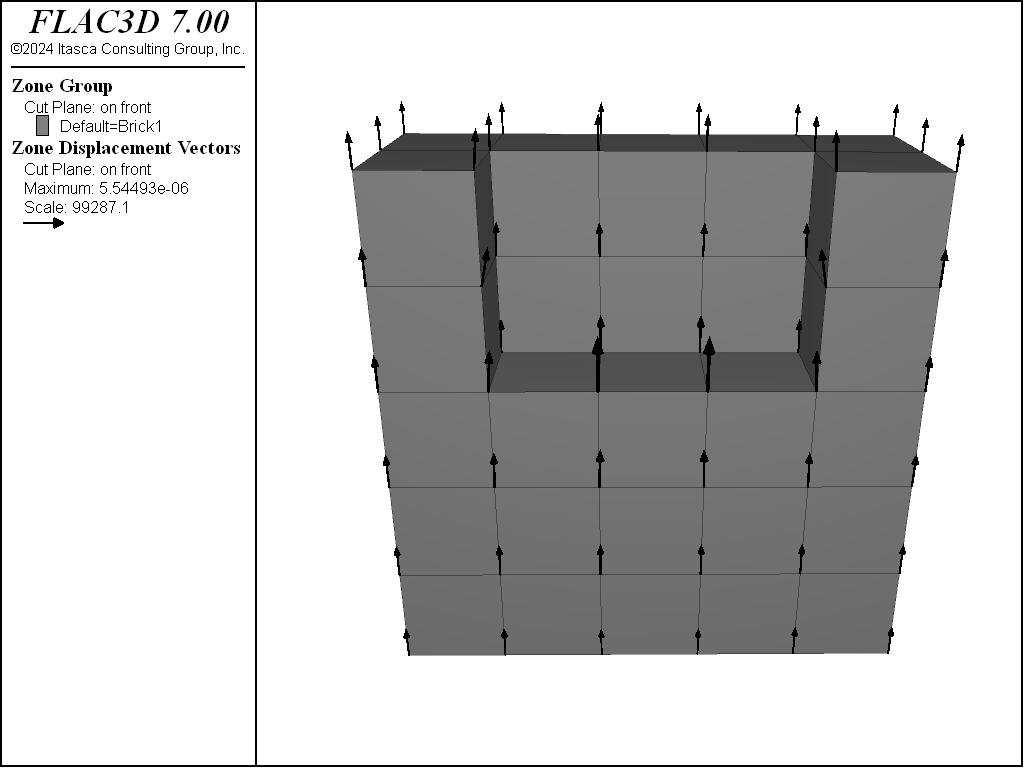
Figure 1: Uplift when material is removed
The difficulty encountered in running this data file can be eliminated by fixing the bottom boundary, rather than supporting it with stresses. Artificial Boundaries contains information relating to the location of such artificial boundaries.
Finally, the stress boundary affects all degrees-of-freedom. Velocity boundary conditions must, therefore, be prescribed after stress boundary conditions affecting the same boundary corners. If the stress boundary is applied after the velocity boundary, the effect of the prescribed velocity will be lost. The next example demonstrates this problem.
Mixing stress and velocity boundary conditions
model new
model large-strain on

block create brick 0,10  0,10  0,10
;
block zone generate edgelength 2.0
;
block zone cmodel assign el
block zone prop  dens 1000 bulk 8e9 shear 5e9
;
block gridpoint apply vel-z 0 range pos-z 0.0 ; should be AFTER stress BC
block face apply stress -1e5,0,0 0,0,0 range pos-x  0.0
block face apply stress -1e5,0,0 0,0,0 range pos-x 10.0
block face apply stress 0,-1e5,0 0,0,0 range pos-y  0.0
block face apply stress 0,-1e5,0 0,0,0 range pos-y  10.0
block face apply stress 0,0,-2e5 0,0,0 range pos-z 10.0
;
block hist disp-z pos 0,0,0
model step 100
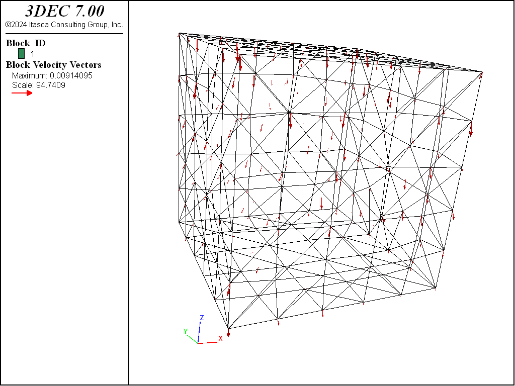
Figure 2: Mixing stress and velocity boundary conditions
The fixed \(z\)-velocity boundary condition along the bottom boundary of the model is removed along the bottom edges of the block when the stress boundaries are applied. These points move downward, as indicated by the velocity vector plot in the figure above, when the model is loaded.
| Was this helpful? ... | 3DEC © 2019, Itasca | Updated: Feb 25, 2024 |