IMASS Model**
Note
**This model requires separate license.
Introduction
The original CaveHoek constitutive model (first appearing in 2010, Pierce 2013) has undergone numerous revisions and enhancements. In terms of strength envelopes, CaveHoek is characterized by two bounding yield surfaces (peak and residual) as shown in Figure 1. Material softening from peak to residual values was controlled by accumulated plastic shear strain. After many successful projects and new discoveries about brittle rock behavior, a new strain-softening model has been created. This new constitutive model is named IMASS (Itasca Model for Advanced Strain Softening). IMASS (Ghazvinian et al., 2020) contains a two-mode softening of yield surfaces as shown in Figure 2. In addition, IMASS material properties have new and unique names when compared to the original CaveHoek. IMASS uses the latest Itasca constitutive model framework and techniques for apex correction, automatic testing, and property updates and management. This document describes IMASS properties and provides several example test cases illustrating IMASS material response.
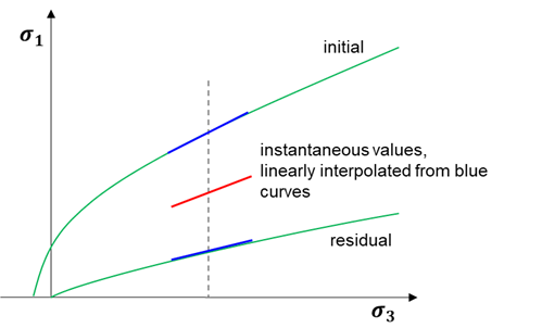
Figure 1: CaveHoek initial (peak) and residual yield surfaces shown in green.
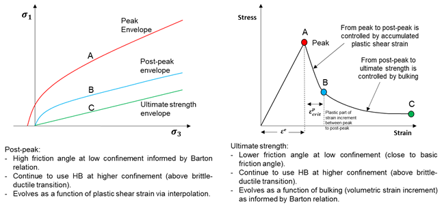
Figure 2: IMASS constitutive model, yield surfaces (left) and material response (right).
IMASS Constitutive Model
A numerical model that represents the damage around an excavation, slope, or caving process must account for the progressive failure and disintegration of the rock mass from an intact/jointed condition to a bulked material. Four critical factors that control the overall behavior of the rock mass matrix during this process are described below.
Cohesion and Tension Weakening and Frictional Strengthening
As the rock mass deforms, it undergoes a reduction in strength from its peak in-situ value to a lower residual value. In general, the massive to moderately jointed rock masses weaken by fracturing and the associated loss of cohesion and tensile strength, but they rapidly strengthen when even lightly confined due to a combination of friction mobilization and dilation resulting from bulking of the fractured rock. These mechanisms largely occur in sequence (Kaiser et al., 2015).
Post Peak Brittleness
The rate at which the strength drops from peak to residual is referred to as brittleness. Rocks that maintain their peak strength with continued loading are referred to as perfectly plastic (ductile). Rock masses that instantaneously drop to residual strength properties when they exceed their peak strength are referred to as perfectly brittle. The brittleness controls how fast or slow the stresses are shed away from the yielded rock mass with accumulated strain.
Modulus Softening
The rock mass increases in volume as intact rock blocks fracture, separate, and rotate during the yielding and mobilization process. Along with this bulking, a reduction in modulus is expected to occur. Representation of the decrease in stiffness is crucial for assessing the evolving stress state around the cave and underground openings, because as rock mass dilates/bulks, its potential to carry stress decreases.
Dilational Behavior
Dilation is the change in volume with shear. An accurate assessment and representation of the dilational behavior of a jointed rock mass is essential to predict the correct volume increase during plastic deformation. This will impact the confinement-dependent strength of the rock mass This overall process — loading the rock mass to its peak strength, followed by a post-peak reduction in strength to some residual level with increasing strain — often is termed a “strain-softening” process and is the result of strain-dependent material properties. Itasca’s most advanced strain-softening model (IMASS) is capable of simulating strain-softening behavior and uses a Hoek-Brown criterion for the peak and residual strength.
Model Main Components
The IMASS constitutive model has been developed to represent the rock mass response to stress changes (i.e., rock mass yield, modulus softening, density adjustment, dilation, dilation shutoff, scaling of properties to zone size, cohesion weakening, tension weakening, and frictional strengthening). This constitutive model was developed using strain-softening material models, with strain-dependent properties adjusted to reflect the impacts of dilation and bulking as a result of induced stress changes. This section and the following sub-sections discuss the fundamentals and implementation of IMASS with a two-mode softening of yield surfaces.
Peak Envelope
The IMASS model peak behavior is based on the built-in “modified Hoek-Brown model”, called the mhoek model. This model contains a tensile strength limit similar to that used by the Mohr-Coulomb model, because the classic Hoek-Brown failure criteria (Hoek et al., 2002) works well at higher confining stress states but can produce excessive dilation at low confinement or under tensile-stress conditions.
The GSI, \(m_i\), and UCS parameters control the shape of the peak Hoek-Brown envelope, which is defined by the following equations (Hoek et al., 2002):
where
Residual Envelopes
Residual envelopes and rock mass softening after reaching peak envelope is a major component of IMASS that is described in detail in Cohesion Weakening Frictional Strengthening Behavior.
Elastic Properties
The intact Young’s modulus (\(E_i\)) is used to calculate the rock mass Young’s modulus (\(E_{rm}\)), using Hoek and Diederichs’ (2006) equation, which governs the rock mass elastic behavior:
Poisson’s ratio is defined as a function of GSI as:
Tensile Strength Envelope
The Hoek-Brown envelope is extended, for a tensile \(\sigma_3\), by a combination of the Mohr-Coulomb envelope (tangent to Hoek-Brown at \(\sigma_3\) = 0) and a tensile cutoff at \(\sigma_3 = -s\sigma_{ci}/m_b\).
Bulking Behavior
The bulking factor or volumetric strain increment (VSI) is defined by:
where \(\Delta V\) is the change in volume (positive = expansion), \(V_i\) is the initial volume, and n is porosity. The initial bulking factor is commonly assumed to be equal to 0 for an undisturbed and unbulked rock. Maximum VSI is the volumetric strain increment value at which the rock mass is considered to have fully bulked.
The bulking factor or VSI is an integral component of IMASS that allows for large-strain processes to control the softening/weakening of strain-dependent properties. For instance, the transition from post-peak envelope to ultimate strength envelope, modulus softening, density adjustment, and dilation shut off are all controlled by VSI in IMASS.
The Hoek-Brown strength envelope only considers the response of the rock mass up to the point of failure. The post peak behavior, which is believed to exert a strong control on rock mass response to stress changes (e.g., due to mining), is not described in this criterion. In order to do this, separate consideration of the post-peak behavior is required.
Cohesion Weakening Frictional Strengthening Behavior
In IMASS, damage, disturbance and the associated loss of strength (i.e. “softening/weakening”) is captured in two phases:
- During Phase 1:
- Damage is the result of fracturing of intact rock due to stress changes. This causes only small (negligible) increases in porosity and permeability.
- Loss of strength results from small-strain processes.
- The numerical assessment of damage is dependent on the accumulation of plastic shear strain. Phase 1 ends when the rock mass reaches the “critical plastic shear strain” and its strength equals the post-peak strength.
- During Phase 2:
- Additional straining and disturbance are the result of rearrangement of rock blocks and cause a significant increase in porosity (up to 40%) and permeability.
- Loss of strength results from large-strain processes.
- The numerical assessment of disturbance is dependent on the accumulation of volumetric strain. Phase 2 ends when the rock mass has reached the “maximum volumetric strain”. At this point, the rock mass has reached its ultimate residual strength and its strength won’t evolve further with additional straining.
Strength Envelopes
Strength weakening in the IMASS constitutive model is defined by three Hoek-Brown strength envelopes, as shown in Figure 3 a peak envelope and two residual strength envelopes (post-peak and ultimate strength). The peak strength envelope (green curve) parameters \(m_b\), s, and a (parameters calc_stren_mb, calc_stren_s, and calc_stren_a in IMASS) are calculated from the classic Hoek-Brown equations based on GSI (in_stren_gsi) and intact rock parameters UCS and \(m_i\) (in_stren_ucsi and in_stren_mi) presented above (see Figure 1 through Figure 4). The Hoek-Brown (H-B) parameters of the residual strength envelopes (red and blue curves) are selected to approximate the peak shear strength for rockfill material as defined by Barton & Kjaernsli (1981):
where \(\tau\) is shear strength, \(\sigma_n\) is the normal stress, \(R\) is equivalent roughness (see Figure 4 ), \(R\) is the rock block strength, and \(\phi_b\) (in_weak_phib) is the basic friction angle for the rock blocks.
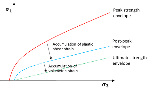
Figure 3: IMASS strength envelopes.
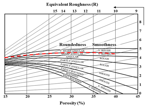
Figure 4: Equivalent roughness of an assembly of rock fragments based on porosity and fragment roundedness/smoothness (Barton & Kjaernsli, 1981).
The first residual strength envelope (the red curve in Figure 3, which is referred to as the post-peak envelope in this document) represents the post-peak strength. At this point, the rock mass is assumed to have undergone fracturing, but the resulting rock fragments are still fully interlocked, and hence, porosity is considered to be zero.
The second residual strength envelope (the blue curve in Figure 3, which is referred to as the ultimate strength envelope in this document) represents the ultimate rock mass residual strength. At this point, the degree of rock fragments interlocking is at its minimum, and the porosity is maximized (maximum porosity of 40% is assumed). Ideally, the first and second residual envelopes describe the behavior of cohesionless, perfectly frictional material with different degrees of interlocking.
The R calculation from the monogram based on porosity and roundedness can be approximated with the following equation:
where \(n\) is prosity, \(ri\) is the roundedness index, with \(ri=0\) for partly rounded/smooth blocks, \(ri=1\) for angular/rough blocks, and \(ri=2\) for very sharp, angular/very rough blocks. When the shear strength from the Barton & Kjaernsli (1981) equation is converted to a strength envelope in \(\sigma_1-\sigma_3\) space, it can be approximated by a Hoek-Brown envelope with the following parameters:
where in_weak_phib is equivalent to \(\phi_b\) in Eq. (8) (in degrees and default = 30 deg) and \(n_{max}\) is the maximum porosity considered in the Barton & Kjaernsli (1981) nomogram, or 40%.
The Hoek-Brown approximation of Eq. (8) that is implemented in IMASS assumes formation and interaction of very sharp, angular, and very rough fragments during the course of bulking, from a porosity of 0% to 40% in the Barton & Kjaernsli (1981) nomogram in Figure 4 (shown with the dashed red line). This also takes into account Itasca’s experience in caving simulations whereby having VSI cut-off of 0.67 (corresponding to 40% porosity) is more realistic than allowing the rock mass to bulk up to 45% porosity. Therefore, Eq. (11) can be further simplified to:
The maximum porosity in this equation is fixed at 0.67 . Therefore, to reach the true residual strength for the rock mass, a zone must bulk to 40% porosity. VSI is the current total VSI for a zone that can be monitored with emer_bulking_totvsi in IMASS. It can be seen that \(s\) and \(m_b\) parameters are equal between post-peak and ultimate strength envelopes, and the only parameter that controls the transition between these two is \(a\):
- For the post-peak envelope (red curve), porosity is fixed to be 0 (VSI = 0.67), resulting in \(a\) = 0.6.
- For the ultimate strength envelope (blue curve), the default porosity is assumed to be 40% (VSI = 0.67), resulting in \(a\) = 0.85.
Note that the maximum bulking capacity of the rock mass can be controlled with in_bulking_maxtotvsi to a value below 0.67. Lowering the maximum allowable VSI for the rock mass would allow for partial weakening of the residual strength envelope between the upper boundary defined by \(a\) = 0.6 and a lower boundary defined by \(a\) = 0.85 (for in_bulking_maxtotvsi = 0.67).
The defined Hoek-Brown parameters for the residual envelopes would result in the following:
- Zero or near zero apparent cohesion and a high friction angle at low confinement for the post-peak envelope, therefore mimicking the cohesion-weakening, frictional-strengthening behavior for the rock mass as it transitions from the peak envelope to post-peak.
- Lower friction angle at low confinement for the ultimate strength envelope. This allows for gradual reduction of the rock mass friction angle from its mobilized post-peak value to the ultimate residual state with increasing porosity (bulking).
- Both post-peak and ultimate strength envelopes continue to use the peak Hoek-Brown envelope at higher confinement (above brittle-ductile transition, see Transition between Peak and Post-Peak Envelopes.
Transition between Peak and Post-Peak Envelopes
When yielding occurs, the instantaneous cohesion weakens linearly from the peak surface to post-peak (zero cohesion when unconfined) with accumulated plastic shear strain (second invariant of the deviatoric plastic strain tensor). The critical shear strain is defined as the total plastic shear strain required to drop the cohesion of a rock mass from peak to zero. At this point, the rock mass is at post-peak strength. The smaller the critical plastic strain, the more brittle a rock mass. Unfortunately, little is known about the critical plastic shear strain required to reach residual strength, particularly on a rock-mass scale. There are very few guidelines for the selection of values for use in modeling.
Some generalizations may be made regarding these effects. For example, a higher-quality rock mass (higher GSI) with greater solid rock volume participating in the failure process often will act in a more brittle fashion, thus having a lower critical strain value. Conversely, a lower-quality rock mass (lower GSI) with higher fracture frequency often will act in a more ductile fashion, thus having a larger value of the critical strain.
An estimate of the relation between the critical strain and GSI was determined by a back analysis of rock mass failure in caves and other openings as part of the MMT project (Lorig, 2000). The estimate provides a starting point for describing the degree of strain-softening to be used in caving simulation:
where \(d\) = zone size in meters.
The presence of zone size within this relation recognizes that the critical strain parameter is zone-size dependent in continuum models, where shearing tends to be resolved in a band approximately one zone thick. By default, in IMASS, a critical plastic shear strain is calculated and stored for each zone based on Eq. (10) using the zone size. A multiplier \(M\) can be applied to the calculated zone-based critical plastic shear strain for refinement of zone brittleness.
Transition between Post-Peak and Ultimate Strength Envelopes
Between the post-peak envelope and ultimate strength envelope, the frictional characteristics of the rock mass is governed by its volumetric strain increment (VSI) instead of plastic shear strain. This replicates the dependency of rockfill shear strength to porosity in the Barton & Kjaernsli (1981) criteria. Since VSI for a zone is not monotonically increasing (unlike plastic shear strain), rock mass strength envelope can weaken or strengthen between post-peak and ultimate strength envelopes as a function of porosity changes. This a powerful feature that allows for capturing strength gain in a rock mass due to recompaction.
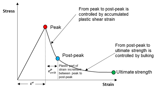
Figure 5: Material response in the IMASS constitutive model.
The rock mass response in terms of stress-strain behavior in IMASS is shown in Figure 5, which summarizes the scale used for softening/weakening of the rock mass between peak to post-peak and then between post-peak and ultimate strength envelopes.
Stress Point Evolution Domains
Fitting Hoek-Brown curves to Barton & Kjaernsli (1981) shear strength criteria can lead to residual and peak strength envelopes crossing in principal stress space at relatively high confinements, depending on the rock mass input properties. To capture a reliable brittle-ductile transition for the rock mass, it is critical to properly account for zone stress evolution and correction in different domains defined by the confining stresses at which the strength envelopes cross one another.
The behavior of three points (A, B, and C) representing different confinement domains in IMASS stress space is shown in Figure 6 and briefly described here. If a stress point is found outside of the peak envelope, somewhere near A, the material yields, the stress point is moved to the peak envelope, and the material accumulates some plastic shear strain. When the stress point is found outside the yield surface during another cycle, instantaneous cohesion and friction angles are calculated (tangent line to the peak envelope at the stress point’s \(\sigma_3\) value, called cohesion_peak and friction_peak). A new yield surface is calculated by linearly interpolating the accumulated plastic shear strain as a parameter between cohesion_peak and cohesion_postpeak and friction_peak and friction_postpeak. The stress point is moved to this new yield surface and more plastic shear strain is accumulated. Eventually, stress point A might reach the post-peak envelope. When this occurs, the strength characteristics of the material start to be governed by its volumetric strain increment (VSI) instead of plastic shear strain. The evolution of friction and apparent cohesion from the post-peak envelope to the ultimate strength envelope is linearly interpolated by using VSI as a parameter between instantaneous cohesion and the friction angle of the two envelopes at the stress point’s \(\sigma_3\) value. The interpolation assumes VSI is equal to zero and 0.67 at the post peak envelope and ultimate strength envelope (40% porosity), respectively.
Yield surfaces of stress point B evolve from the peak Hoek-Brown surface directly to the ultimate residual strength envelope based on VSI and the same rules as above (eliminating the post-peak envelope in the calculations).
Stress point C is simply moved to the Hoek-Brown yield surface (plastic shear strain and VSI are accumulated). However, in that region, the material does not weaken and behaves perfectly plastic. This allows reproduction of the brittle to ductile transition that is observed in rock masses at high confinement. In general, hardening is not allowed in IMASS implementation when residual strength envelopes cross the peak yield surface.
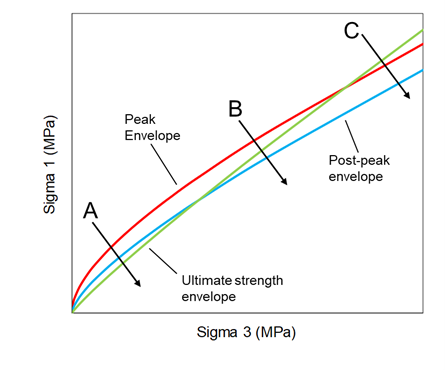
Figure 6: IMASS stress point evolution domains.
Mohr-Coulomb Fit
Linear interpolation of Hoek-Brown \(m\), \(s\), and \(a\) parameters does not give a smooth transition of the strength envelope between peak and residual strength. Therefore, IMASS performs a linear interpolation directly between the linear Mohr-Coulomb fits at the three defining yield surfaces for the rock mass based on the current stress state. The Mohr-Coulomb approximation of the Hoek-Brown strength envelopes is performed over a range bounded by the current zone stress level (\(\sigma_3\)) and \(\sigma_3+\Delta \sigma_3\), where \(\Delta \sigma_3\) = 10 Pa.
Tension Weakening and Tension Cutoff
The peak tensile strength for a rock mass in IMASS is adopted as the minimum of:
- the tensile strength determined by the HB model (\(sUCS⁄m_b\) );
- the tensile strength determined by the equivalent MC strength line (\(c⁄\tan{\phi}\)); and
- the input tensile strength, either by a scalar value (calc_stren_tension), or by a table-like property (in_weak_tabletension).
With the growth of new fractures during shear, the tensile strength of every zone is linearly weakened with the increase of its accumulated plastic shear strain (see Figure 7 a) until it reaches its post-peak value (note that post-peak tensile strength is 0 with the default residual parameters).
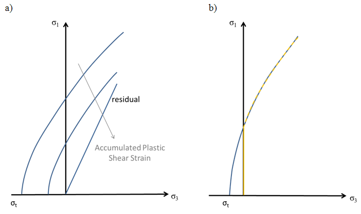
Figure 7: Graphical representation of Hoek-Brown failure envelope with tension weakening: (a) Tensile strength degradation occurring with accumulated plastic shear strain. (b) Sudden loss of tensile strength during tensile failure (yellow line represents tensile shutoff).
The softening of a rock mass can be attributed to strain-based damage manifesting as intact rock block damage (accumulation of micro-cracks) and joint slip/dislocation and/or extension. So far, through the standard strain-softening relation, only shear softening has been considered. However, shear failure is only one yielding mechanism for a rock mass. Tensile failure can also be expected. Brown (2003) has shown this within the conceptual model of caving based on the review of fracture models within a cave mine.
Tensile failure is dominated by the existence of pre-existing fractures in the rock mass. Because there is no consideration of the joint orientation in a strain-softening model, the impact of independent tensile failure due to pre-existing joints must be accounted for in another way. Figure 8 shows how it is feasible that tension can soften independently of cohesion when a tensile failure mechanism is simulated in a rock mass.
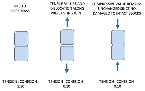
Figure 8: Schematic diagram of tensile failure that does not affect cohesive strength.
This phenomenon has previously been described by Pine et al. (2007): “Crack growth orthogonal to the direction of dilation in a compressive stress field does not immediately produce a mechanical instability, as observed in tensile fields … It is this stable fracture process in compression that results in large differences between tensile and compressive strengths.”
The mechanism of independent tensile softening is implemented in IMASS, i.e., in addition to softening tension and cohesion at the same rate based on plastic shear strain, tension is allowed to soften independently of the cohesion in the instance of a tensile yield state within a zone. For implementation of such a mechanism in IMASS, the rock mass is treated perfectly brittle in tension. Therefore, any time a zone reaches its peak tensile strength, it is presumed to permanently weaken to zero tensile strength in a perfectly brittle fashion as represented in Figure 8 b. If that happens during the simulation, then the emer_weak_istenweak is set to a value greater than zero (and less than or equal to 1) for that zone (instead of zero). Note that a zone that has not failed in tension can reach a zero tensile strength only by tension weakening due to accumulated plastic shear strain; in that case, the emer_weak_istenweak parameter is still equal to zero. The perfectly brittle response of a zone in tension can be turned off by setting the flag_weak_tencut to false. In that case, a perfectly plastic behavior is assumed for a zone in tension when that zone reaches its peak tensile strength, unless it progressively decreases by accumulation of plastic shear strain or if a table that correlates tension weakening to accumulated plastic tensile strain is assigned to the zone (in_weak_tabletension).
Dilation Angle
During mining operations such as caving, the rock mass will increase in volume (or bulk) due to dilation under shear, or due to volumetric expansion under tension. Thus, the specification of a dilation angle within the numerical model is important, as it controls the rate of bulking during shearing, which is a natural consequence of advance or differential draw (in caving). Figure 9 shows non-uniform bulking in the mobilized zone as a consequence of the two bulking mechanisms acting simultaneously within the model.
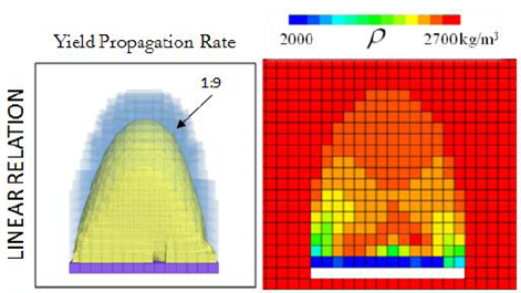
Figure 9: Non-uniform bulking in the mobilized zone (Sainsbury, 2010).
Within IMASS, dilation angle is set as a standard material property and drops to zero once the user-defined maximum bulking factor is reached. This prevents zones from expanding to unrealistic levels during shear. A constant dilation angle can be assigned to the rock mass (i.e., equal everywhere) based on the available guidelines such as those provided by Hoek and Brown (1997). Alternatively, a more advanced dilation model is available that constantly updates the dilation angle for each zone as a function of confining stress and porosity (or VSI). Figure 10 presents a graphical representation of this model as implemented in IMASS. In this piece-wise model, the dilation angles at zero porosity are informed by the results of Bonded Block Modeling (BBM) (Garza-Cruz et al., 2019). The linear section of the model between 15% to 45% porosity is equivalent to the dilatant part of Barton’s approximation of friction angle for rockfill (i.e., \(R\log{S/\sigma_n}\)). Finally, a function that exponentially decays with porosity connects the two parts of the model between 0 and 15% porosity.
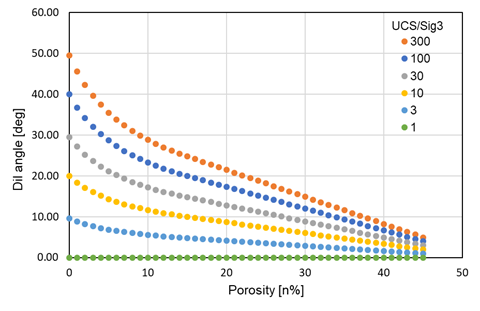
Figure 10: Dilation model in IMASS as a function of confining stress and porosity.
The necessity for assembling this model stems from the fact that all of the available empirical dilation models based on laboratory test data, such as those proposed by Walton and Diederichs (2015) and Alejano and Alonso (2005), only apply to rock deformations of the order of thousands of microstrains. This level of strain corresponds only to rock mass softening from peak to post-peak envelopes; therefore, these empirical models do not provide any insight into the estimation of dilation angle at high porosities (between post-peak and ultimate strength envelopes).
Modulus Softening
As a rock mass bulks via shear or tension, it is expected to experience a drop in modulus. Representation of this softening is required in order to properly capture how new loads are carried in bulked regions. In addition, it is necessary to allow for modulus hardening that can occur when stresses are shed back onto bulked regions (inducing recompaction).
The results of laboratory testing by Pappas and Mark (1993) (Figure 11) show that the modulus of rock drops in a nonlinear fashion with increased bulking, and that the rate of modulus change is a function of fragment shape and intact strength. Based on the results of these tests, they developed a series of equations that can be used to estimate modulus as a function of bulking factor (BF), the uniaxial compressive strength (UCS, in psi) of the intact rock fragments, as well as the aspect ratio of the fragments denoted by X1 and X2 in Table 1. Note that the Pappas and Mark (1993) definition of BF (BF = 1 + broken-rock bulking factor, defined here as B) is different from what is used typically in caving. The chart shown in Figure 12 can be used to estimate the thickness-to-width (aspect) ratio (specified as 0.6 in IMASS).
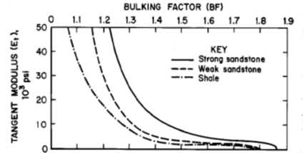
Figure 11: Best-fit tangent modulus (in psi) versus void ratio for all rock types tested by Pappas and Mark (1993). The y-axis (modulus) limit of 50,000 psi in this plot is equal to 345 MPa. The lower x-axis (void ratio) limit of 1.9 is equivalent to a porosity of 47%.
| Tangent (\(E_t\)) Modulus at Various Bulking Factors (BF) (Pappas and Mark 1993) | |
| BF = 1.25 | \(E_t = 2.49 X_1 + 41200 X_2 - 24800\) |
| BF = 1.30 | \(E_t = 1.76 X_1 + 23800 X_2 - 15700\) |
| BF = 1.25 | \(E_t = 1.32 X_1 + 16300 X_2 - 11400\) |
| BF = 1.40 | \(E_t = 0.933 X_1 + 11300 X_2 - 7900\) |
| BF = 1.50 | \(E_t = 0.568 X_1 + 6900 X_2 - 500\) |
Note
This is based on laboratory oedometer tests on materials of varying bulking factor (BF), intact strength and fragment shape. \(X_1\) is the uniaxial compressive strength (UCS) of the intact rock fragments (in psi); \(X_2\) is the thickness-to-width (aspect) ratio of the fragments.
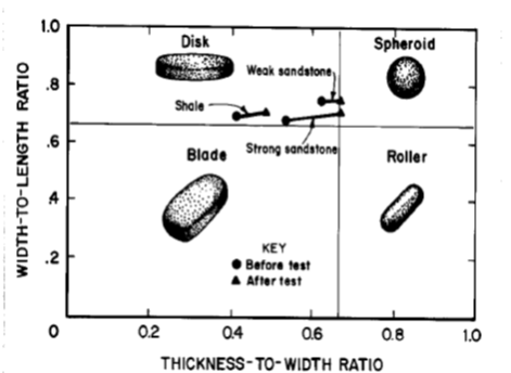
Figure 12: Pappas and Mark (1993) chart for estimation of fragment thickness-to-width ratio.
The modulus softening equations listed in Table 1 for different BFs can be summarized in one equation by fitting curves to the X1-X2 coefficients and constants. The curves are expressed as exponential functions of VSI (bulking or B):
where
During simulation, the broken-rock bulking factor in each zone is given by its VSI. If the broken-rock bulking factor is greater than 0.25, the Pappas and Mark equation is used to establish a new tangent modulus for the zone based on the user-defined UCS, shape factor (0.6 in IMASS), and BF (caved rock bulking factor + 1). For broken-rock bulking factors less than 0.25, the tangent modulus is calculated through interpolation between the in-situ rock mass modulus and the Pappas and Mark modulus corresponding to a broken-rock bulking factor of 0.25. Figure 13 through Figure 14 show the relations in graphical form as a function of initial modulus and UCS. Because the modulus is updated constantly via the zone-based VSI, it allows for both modulus softening (during bulking) and modulus hardening (e.g., during re-compaction of exhausted or undrawn parts of the cave).
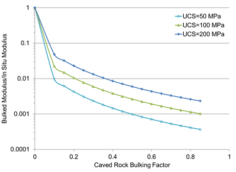
Figure 13: Sensitivity of Pappas and Mark modulus-softening relations to UCS (\(E_i\) = 10 GPa, aspect ratio = 0.5).
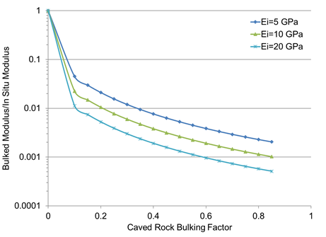
Figure 14: Sensitivity of Pappas and Mark modulus-softening relations to initial rock-mass modulus, \(E_i\) (UCS = 100 MPa, aspect ratio = 0.5).
Density Adjustment
Due to the large displacements involved in caving, a caving simulation run in large-strain mode (i.e., node coordinates are updated based on calculated strain) would involve extreme mesh deformation. While it may be possible to employ dynamic remeshing techniques to accommodate this, it has been shown that caving can be simulated in small-strain mode as long as mass balance is maintained. In small-strain mode, node coordinates are not updated and the zone density is adjusted continuously in IMASS to reflect the volumetric changes that accompany bulking, according to the following relation:
where
\(\rho_d\) = dry density of caved rock;
\(\rho_s\) = solid density of in-situ rock;
B = bulking factor;
1 + B = swell factor; and
n = porosity.
By default, density adjustment is not performed in IMASS (flag_bulking_denadj = off). It can be activated by setting flag_bulking_denadj to true/on/yes, in which case, IMASS will adjust zone density based on the current value of VSI.
Ubiquitous Joints
To keep IMASS implementation clean, the ubiquitous joint logic is borrowed from FLAC3D within the hierarchy structure.
Tensile strength, cohesion, and friction angle control the Mohr-Coulomb envelope for the ubiquitous joints; dip and dip direction are set equal to those of structures or joints to represent their true orientation.
Single Residual Envelope Implementation (Similar To Cavehoek) In IMASS
IMASS provides the user with the option to choose between a single residual envelope approach (similar to the CaveHoek approach) or the Barton shear strength approach in which the post-peak behavior is defined by two residual envelopes bounded by 0 and a higher porosity (e.g., 40%) for the rock mass. The default method to simulate post-peak in IMASS is the Barton shear strength criteria (flag_weak_barton = true). While there are some minor differences between an IMASS model with one residual envelope and CaveHoek (more details on fundamental differences are presented in Differences between the Single Residual Envelope Implementation in IMASS and the CaveHoek Model), this option would streamline the comparison between the IMASS and CaveHoek results if necessary, within one constitutive model. It also provides the flexibility to turn on the one residual envelope depending on the application (e.g., when large strains are not anticipated).
To switch to the post-peak simulation approach similar to CaveHoek, flag_weak_barton needs to be set to false. The residual envelope is then defined by in_weak_chmbr (default 4.33), in_weak_char (default 1.0), and a residual s value that is set to zero and can’t be modified by the user. This residual envelope is treated similarly to the post-peak envelope in a two-residual implementation, meaning that weakening between the peak strength envelope and the residual envelope is controlled by the accumulated plastic shear strain. The VSI-based modulus and density adjustment, dilation model, and dilation shut-off remain unchanged.
Differences between the Single Residual Envelope Implementation in IMASS and the CaveHoek Model
The fundamental differences between CaveHoek and IMASS are the updated yield surfaces and new property names. Additional differences include the following.
- IMASS does not allow strength hardening when the residual envelopes cross the peak envelope (CaveHoek does).
- IMASS, by default, uses a constant dilation angle specified by property in_bulking_dil before reaching the maximum VSI. At this point, an experimental dilation model as described in Modulus Softening is implemented in IMASS; however, this model is different from those available in CaveHoek (see hb_doption in CaveHoek).
- In IMASS, the calculated properties are updated automatically when the input properties for given zones are updated (see PROPERTIES IN *IMASS*).
It should be noted that despite implementing the single residual envelope mode in IMASS, the results might slightly differ from those obtained from CaveHoek due to a more advanced apex correction in IMASS and other minor differences between the two models, such as allowing/limiting strength hardening when the peak and residual envelopes cross each other.
Sloss, an indicator for damage in IMASS
Sloss is an indicator of damage in IMASS that can be used to evaluate the amount of softening/weakening that a rock mass has gone through. Sloss varies between [-1, 1].
Between Peak and post-peak envelopes:
Between post-peak and ultimate strength envelopes:
Figure 15 schematically represents sloss for different degrees of damage and disturbance in a rock mass. At “C” the rock mass is assumed to have undergone fracturing, but the resulting rock fragments are still fully interlocked (cohesion in the rock mass is completely lost but friction is high). At this point the stress is above the spalling or fracturing strength of the rock. However, experience has shown that the underground opening is stable with minimal support. At “D” the degree of rock fragments interlocking is at its minimum and the porosity is maximized. Unlined shafts or minimally supported drifts at this stress state are considered unserviceable. If sloss is calibrated to field observations in terms of damage, it can be a powerful tool for prediction of the serviceability and stability of the structure.
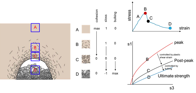
Figure 15: Schematic representation of sloss for various degrees of damage in a rock mass (cave schematic after Potvin 2018).
Examples using IMASS
Properties In IMASS
IMASS properties have been logically grouped as shown in Table 2. Property names have three parts, the first two parts corresponding to the groups in Table 2. The first piece of the property name is either in_, calc_, emer_, or flag_ to distinguish inputs, calculated values, emergent values, or flags, respectively. These categories are columns in Table 2. Row categories group properties based on peak strength, modulus, strength weakening, dilation, bulking and modulus softening, stress at failure, and ubiquitous joints. These groupings form the second portion of the property name (stren_, mod_, weak_, bulking_, sfail_, uj_, respectively). The remaining portion of a property name is a specific descriptive name such as GSI or youngintact. Without the two prefixes, the third portion of the property names are somewhat similar to many of the property names used in the original CaveHoek model. Property names are described in detail in IMASS Properties.
The italicized properties in Table 2 are the minimum input properties that are required for IMASS. In general, the Input properties and Flags are parameters provided by the user. Calculated properties are the sets of parameters that are initially calculated by IMASS based on the Input properties and Flags. Every time the Input properties or Flags are assigned or updated by the user, the calculated properties will be updated automatically by IMASS. The Calculated properties are generally not modifiable; however, there are some exceptions that will be listed in IMASS Properties. Emergent properties are the sets of parameters that evolve as a consequence of stress changes in the model. Those parameters are not modifiable by the user.
| Flags/Inputs | Calculated | Emergent | |
|---|---|---|---|
| Peak | flag_stren_mod(off) | calc_stren_global | |
| strength | in_stren_gsi | calc_stren_tension | |
| in_stren_mi | calc_stren_ucsrm | ||
| in_stren_ucsi | calc_stren_mb | ||
| calc_stren_s | |||
| calc_stren_a | |||
| Modulus | in_mod_youngintact | calc_mod_youngrm | emer_mod_young |
| calc_mod_poisson | |||
| Strength | flag_weak_barton(on) | calc_weak_ecrit | emer_weak_sloss |
| weakening | flag_weak_tencut(on) | calc_weak_zsize | emer_weak_esplastic |
| in_weak_multecrit | emer_weak_istenweak | ||
| in_weak_chmbr(4.33) | emer_stren_mcfric | ||
| in_weak_char(1.0) | emer_stren _mccoh | ||
| in_weak_phib(30) | emer_stren_tension | ||
| in_weak_sloss(1.0) | |||
| in_weak_tabletension | |||
| Dilation/ | flag_bulking_denadj | emer_bulking_mcdil | |
| bulking & | flag_bulking_modsoft | emer_bulking_den | |
| modulus | in_bulking_den | emer_bulking_totvsi | |
| softening | in_bulking_dil | ||
| in_bulking_targetvsi | |||
| in_bulking_maxtotvsi(2/3) | |||
| Stress at | flag_sfail_failtrack(off) | emer_sfail_pmax | |
| failure | emer_sfail_plungepmax | ||
| emer_sfail_trendpmax | |||
| emer_sfail_pmid | |||
| emer_sfail_plungepmid | |||
| emer_sfail_trendpmid | |||
| emer_sfail_pmin | |||
| emer_sfail_plungepmin | |||
| emer_sfail_trendpmin | |||
| Ubiquitous | flag_uj_usejoints(on) | emer_uj_esplastic | |
| joint | in_uj_jcoh | ||
| in_uj_jdil | |||
| in_uj_jfric | |||
| in_uj_jten | |||
| in_uj_jdip | |||
| in_uj_jddirection(on) | |||
| in_uj_jnx | |||
| in_uj_jny | |||
| in_uj_jnz |
Unit System
IMASS uses a single set of SI units as listed in Table 3. Do not use any other system of units in this model.
| Length | \(m\) |
| Density | \(kg/m^3\) |
| Force | \(N\) |
| Stress/Pressure/Modulus | \(Pa\) |
| Gravity | \(m/s^2\) |
Resetting Properties
The calculated properties (for instance calc_stren_mb, calc_stren_s and calc_stren_a) are automatically updated when new values are specified for IMASS input parameters such as in_stren_gsi, and in_stren_mi. This has been done to avoid the confusion that was experienced by some users of CaveHoek, whereby hb_mmi, hb_ssi, hb_aai had to be set to -1 when new values were being specified for the input parameters.
The following points should be kept in mind when resetting properties in IMASS:
- Strength properties of a zone between post-peak and ultimate strength envelope can be reset to their peak values by setting in_weak_sloss = +1.0. However, if a zone has accumulated sufficient plastic shear strain to be placed past the post-peak envelope whereby the zone strength properties are controlled by VSI, the input properties for the zone have to be redefined to restore it to its peak strength properties. It should be kept in mind that VSI is a FLAC3D property (not an IMASS property) and non-reversible. Therefore, even by redefining the input properties for a zone, some VSI-dependent elastic properties or density might not fully recover to their initial values.
- If the residual state of a zone is changed iteratively using in_weak_sloss or in_bulking_targetvsi, IMASS will not notice a change if those parameters are reset to a value that is already assigned to them (or is their default value). For instance, if in_bulking_targetvsi is set to 0.5 in cycle 1 and in cycle 100 in_bulking_targetvsi is again reset to 0.5, IMASS will not realize that.
References
Hoek, E., C. Carranza-Torres and B. Corkum. (2002) “Hoek-Brown Failure Criterion - 2002 Edition,” in NARMS-TAC 2002: Mining and Tunneling Innovation and Opportunity, Vol. 1, 267–273, R. Hammah, W. Bawden, J. Curran, and M. Telesnicki, Eds. Toronto: University of Toronto Press.
Hoek, E., and M. S. Diederichs. (2006) “Empirical Estimation of Rock Mass Modulus,” Int. J Rock Mech. Min. Sci, 43, 203–215.
Lorig, L & Pierce, M (2000) “Methodology and Guidelines for Numerical Modelling of Undercut and Extraction Level Behavior in Caving Mines,” Itasca Consulting Group Inc., Report to the International Caving Study.
Pappas, D., and C. Mark. (1993) “Behavior of Simulated Longwall Gob Material,” Report of Investigations, 9458 USBM.
Hoek, E., and E. T. Brown. (1997) “Practical Estimates of Rock Mass Strength,” Int. J. Rock Mech. Min. Sci., 34(8), 1165–1186.
Pierce, M. (2013) “Numerical Modeling of Rock Mass Weakening, Bulking and Softening Associated with Cave Mining,” ARMA E-Newsletter Spring 2013, (9).
Barton, N., and B. Kjaernsli. (1981) “Shear Strength of Rockfill,” J. Geotech. Engr., GT7, 873–891.
Cumming-Potvin, D, Wesseloo, J, Jacobsz, SW & Kearsley, E (2018), “A re-evaluation of the conceptual model of caving mechanics”, in Y Potvin & J Jakubec (eds), Proceedings of the Fourth International Symposium on Block and Sublevel Caving, Australian Centre for Geomechanics, Perth, pp. 179-190.
Ghazvinian, E., Garza-Cruz, T., Bouzeran, L., Fuenzalida, M., Cheng, Z., Cancino, C., and Pierce M. (2020). “Theory and Implementation of the Itasca Constitutive Model for Advanced Strain Softening (IMASS),” in Proceedings Eighth International Conference and Exhibition on Mass Mining (MassMin 2020): Santiago.
Sainsbury, B. (2010) “Sensitivities in the numerical assessment of cave propagation” in Caving 2010: Second International Symposium on Block and Sublevel Caving. 20–22 April 2010, Australian Centre for Geomechanics.
imass Model Properties
Use the following keywords with the zone property (FLAC3D) or block zone property (3DEC) command to set these properties of the IMASS model.
- imass
Peak Strength
- flag_stren_mod b
Flag, the default is off. Set this to on to manually define the peak Hoek-Brown parameters calc_stren_mb, calc_stren_s and calc_stren_a.
- in_stren_gsi f
Geological Strength Index, GSI. This is one of primary properties with allowable input values between 0 and 100.
- in_stren_mi f
Hoek-Brown parameter for intact rock, \(m_i\). This is one of primary properties and must be a positive input value.
- in_stren_ucsi f
Uniaxial compressive strength (UCS) of intact rock [Pa], \(\sigma_{ci}\). This is one of primary properties and must be a positive input value.
- calc_stren_tension f (r)
Tensile strength [Pa]. This value equals to \(s \sigma_{ci}/m_b\).
- calc_stren_ucsrm f (r)
Uniaxial compressive strength [Pa]. This value equals to \(s^a\sigma_{ci}\).
Modulus
- in_mod_youngintact f
Young’s modulus of intact rock [Pa], \(E_i\). This is one of primary properties and must be a positive input value.
- calc_mod_poisson f (r)
Poisson’s ratio estimated for the rock mass. See Equation (6). This usually is automatically calculated based on GSI by default. If this parameter is specified before initialization of calculated properties by IMASS, then IMASS will not automatically calculate this parameter. Note that if it has been (or the user input) a positive non-zero value, the Poisson ratio will not recalculated by Equation (6). To make it recalculated by Equation (6), just input a zero value.
- emer_mod_young f (r)
Current Young’s modulus of the rock mass [Pa].
Strength Weakening
- flag_weak_barton b (a)
Flag, the default is on. Set this to off to disable Barton & Kjaernsli (1981) shear strength criteria (two residual envelopes) to be used for post-peak behavior and use the single residual method instead.
- flag_weak_tencut b (a)
Flag, the default is on. Set this to off to disable the tension cutoff option. A material is deemed to be tension weakened if it exceeds its tensile strength in at least one of the zone’s tet overlays. If a material is tension weakened (property emer_weak_istenweak is calculated by IMASS as the ratio of total volume of tet overlays failed in tension to the overall zone volume) and if flag_weak_tencut = on, material tensile strength will be set to zero.
- in_weak_multecrit f (a)
A multiplier for critical plastic shear strain for the matrix material. This property must be assigned by the user. Critical strain (Equation 13) is initially calculated based on input properties as (12.5 - 0.125 * GSI + 1.0e-5) / (100.0 * calc_weak_zsize) and then multiplied directly by in_weak_multecrit; the resulting product is stored in variable calc_weak_ecrit. Material can be made to have a more brittle response by setting in_weak_mult_ecrit to a value less than 1.0 (and greater than 0.0) or more ductile by setting in_weak_multecrit to a value > 1.0
- in_weak_chmbr f (a)
Residual value of Hoek-Brown parameter \(m_{br}\) when only one residual strength curve is used (flag_weak_barton = off). The default is 4.33.
- in_weak_char f (a)
Residual value of Hoek-Brown parameter \(a_r\) when only one residual strength curve is used (flag_weak_barton = off). The default is 1.0.
- in_weak_phib f (a)
Basic friction angle for the rock blocks in Barton & Kjaernsli (1981) shear strength criteria [degrees], \(\phi_b\), see Equation (8). The default is 30.0.
- in_weak_sloss f
Input sloss value to initialize some damage in the rock mass and start from a residual state [dimensionless]. Five rules apply to using this property:
- The in_weak_sloss should be between -1.0 to 1.0.
- If the zone current sloss (emer_weak_sloss) is between 0.0 and 1.0, then in_weak_sloss = 0 won’t be effective because the zone behavior is controlled by accumulated plastic shear strain.
- If the zone current sloss (emer_weak_sloss) is between -1.0 and 0.0, then an in_weak_sloss > 0 won’t be effective because the strength properties of a zone that is past the post-peak envelope cannot move back to the space between peak and post-peak envelopes.
- If in_weak_sloss is reset to its current value, IMASS won’t notice the change.
- The in_weak_sloss property cannot be used in combination with in_bulking_targetvsi.
- in_weak_tabletension s
Name of the table relating matrix tensile strength to critical plastic tensile strain (emer_weak_etplastic).
- calc_weak_ecrit f (r)
Critical strain for the matrix material [m/m] used for material softening calculations. Critical strain is initially calculated based on input properties as Equation :eq:`modelimasscriticalstrain` and then multiplied directly by in_weak_multecrit; the resulting product is stored in calc_weak_ecrit.
- calc_weak_zsize f (r)
Zone size represented by the cube root of zone volume [m], \(Z\). This is used to calculate the critical strain, see Equation (14). Note that this is a read-only variable.
- emer_weak_esplastic f (r)
Current accumulated plastic shear strain, \(\gamma^p\).
- emer_weak_etplastic f (r)
Current accumulated plastic tensile strain.
- emer_weak_istenweak f (r)
emer_weak_istenweak = 0 initially, but changes to maximum value of 1.0 as material yields in tension. It is calculated as the ratio of total volume of tet overlays in a zone that are yielded in tension to the overall volume of the zone.
- emer_weak_sloss f (r)
Strength loss indicator (\(S_L\)) which varies between +1 and -1 (\(-1 \le S_L \le 1\)). A material which has not yielded has \(S_L = 1\). This value linearly reduces to 0 as a function of \(\gamma^p\). When \(\gamma^p = \gamma_{crit}\), \(S_L = 0\). \(S_L\) linearly varies between 0 and -1 as a function of \(VSI_c\). When \(VSI_c = 2/3\), \(S_L = -1\), therefore if \(VSI_{max} < 2/3\) is specified \(S_L\) can only decrease to a value equal to \(-1.5 VSI_c\) but not -1.
- emer_stren_mcfric f (r)
Current value of friction [degrees]. Calculated for each tet individually in overlays, this reported value is the average value of tet overlays for the zone.
- emer_stren_mccoh f (r)
Current value of cohesion [Pa]. Calculated for each tet individually in overlays, this reported value is the average value of tet overlays for the zone.
- emer_stren_tension f (r)
Current value of tension cutoff [Pa]. Calculated for each tet individually in overlays, this reported value is the average value of tet overlays for the zone.
Dilation, Bulking and Modulus Softening
- flag_bulking_denadj f (a)
Flag, the default is off. When this flag is on, IMASS will adjust zone density based on current value of VSI.
- flag_bulking_modsoft f (a)
Flag, the default is on. Set this to off to disable modulus softening. The fragment aspect ratio for modulus softening calculation is set to 0.6.
- in_bulking_den f (a)
Initial material density [\(kg/m^3\)]. This can be obtained internally from the zone density, which can be set with the command of
zone initialize density. The zone’s density may be altered by IMASS (if flag_bulking_denadj = on).
- in_bulking_dil f (a)
Initial dilation angle [degrees], the default is 10. If inputting a positive value (option 1), this positive constant dilation angle will be used. If inputting a negative value (option 2), the built-in evolving dilation angle will be used (shown in Figure 10). With either dilation option, the dilation angle is set to zero when a user-defined maximum bulking factor (\(VSI_{max}\)) is reached. This prevents zones from expanding to unrealistic levels during shearing.
- in_bulking_targetvsi f (a)
Target bulking factor or VSI (Volumetric Strain Increment), \(VSI_{tgt}\). When in_bulking_targetvsi is specified as a positive value for a zone, the plastic shear strain is set to calc_weak_ecrit for that zone, and it is placed past the post-peak envelope in principal stress space. The VSI for the purpose of strength envelope calculation is assumed to be zero on the post-peak envelope and equal to in_bulking_maxtotvsi on the ultimate strength envelope; therefore, the relative position of the zone between the two residuals is determined based on the specified in_bulking_targetvsi. Setting property in_bulking_targetvsi to a positive value is useful to force a material to start at an accumulated strain level. emer_bulking_totvsi = in_bulking_targetvsi at the beginning of the cycle at which the in_bulking_targetvsi value is specified. A set of rules applies to using this property:
- in_bulking_targetvsi cannot be larger than in_bulking_maxtotvsi.
- If the zone current sloss (emer_weak_sloss) is between 0.0 and 1.0, then in_bulking_targetvsi = 0 won’t be effective because the zone behavior is controlled by accumulated plastic shear strain.
- If in_bulking_targetvsi is reset to its current value, IMASS won’t notice the change.
- in_bulking_targetvsi cannot be used in combination with in_weak_sloss.
- in_bulking_maxtotvsi f (a)
Maximum bulking factor, \(VSI_{max}\). The default is 2/3. After zone’s VSI reaches this limit, the dilation is shut off and density adjustment is terminated. in_bulking_maxtotvsi also controls the extent of strength weakening for the ultimate strength envelope. It can change anywhere between post-peak envelope (in_bulking_maxtotvsi = 0) and a strength envelope corresponding to 40% of rock mass porosity (in_bulking_maxtotvsi = 2/3), which is the default ultimate strength envelope in IMASS.
- emer_stren_mcdil f (r)
Current value of dilation [degrees], calculated for each tet individually in overlays, this reported value is the average value of tet overlays for the zone.
- emer_bulking_den f (r)
Current zone density [\(kg/m^3\)]. The zone’s density may be altered by IMASS, and current zone density is available in properties density and emer_bulking_den. See the in_bulking_den property for additional information.
- emer_bulking_totvsi f (r)
Current total VSI value, \(VSI_c\), used in modulus calculations, density adjustment, dilation model, dilation shut off, and updating the strength envelope between post-peak and ultimate strength. emer_bulking_totvsi = [VSI from zone] + [amount of VSI that is automatically calculated by IMASS from in_bulking_targetvsi if specified].
Stress at Failure
- flag_sfail_failtrack f (a)
Flag, the default is on. Set this to off to disable failure stress tracking. IMASS records trend and plunge of the principal stress direction. Trend = angle in degrees measured clockwise from North (toward the East axis). Plunge = angle in degrees, measured positive downward from the horizontal which is at 0 degrees. In FLAC3D and 3DEC model space, positive y-axis points North, positive x-axis points East, positive z-axis points up. Note FLAC3D and 3DEC use the convention of negative stresses being compressive and tensile stresses being positive. IMASS records and reports the following values for the first subzone (tet) that reaches the specified yielding limit for any given zone.
- emer_sfail_pmax f (r)
Maximum, most positive principal stress [Pa].
- emer_sfail_plungepmax f (r)
Plunge [degrees] of maximum principal stress.
- emer_sfail_trendpmax f (r)
Trend [degrees] of maximum principal stress.
- emer_sfail_pmid f (r)
Intermediate principal stress [Pa].
- emer_sfail_plungepmid f (r)
Plunge [degrees] of intermediate principal stress.
- emer_sfail_trendpmid f (r)
Trend [degrees] of intermediate principal stress.
- emer_sfail_pmin f (r)
Minimum, most negative principal stress [Pa].
- emer_sfail_plungepmin f (r)
Plunge [degrees] of minimum principal stress.
- emer_sfail_trendpmin f (r)
Trend [degrees] of minimum principal stress.
Ubiquitous Joint
IMASS uses the hierarchy approach to borrow the ubiquitous joint logic from FLAC3D. To use joints, property flag_uj_usejoint must be set to on and joint properties must be set. Note all joint properties are initially zero. For weakness plane orientation, specify properties in_uj_jdip and in_uj_jddirection or properties in_uj_jnx, in_uj_jny, and in_uj_jnz (these components of the normal to the weakness plane are not required to be a unit vector, IMASS normalizes them).
- flag_uj_usejoints f (a)
Flag, the default is off. Set this to on if to set ubiquitous joints (ubiquitous joint properties must also be set for this case). Note all joint properties are initially zero. For weakness plane orientation, specify properties in_uj_jdip, in_uj_jddirection or properties in_uj_jnx, in_uj_jny, in_uj_jnz (these components of the normal to the weakness plane are not required to be a unit vector, IMASS normalizes them internally).
- in_uj_jcoh f
Joint cohesion [Pa], \(c_j\)
- in_uj_jfric f
Joint friction angle, \({\phi}_j\)
- in_uj_jdip f
Dip [degrees] of weakness plane, measured positive down from xy plane.
- in_uj_jddirection f
Dip direction [degrees] of weakness plane], measured in xy plane, positive clockwise from positive \(y\)-axis (North) toward positive \(x\)-axis (East).
- in_uj_jnx f
\(x\)-component of the normal direction to the weakness plane \(n_x\).
- in_uj_jny f
\(y\)-component of the normal direction to the weakness plane \(n_y\).
- in_uj_jnz f
\(z\)-component of the normal direction to the weakness plane \(n_z\).
- emer_uj_esplastic f (r)
Accumulated plastic shear strain in the joint.
Development and Version Control
- version i (r)
IMASS is actively used and enhanced through experience and research at Itasca. This read-only property is used by the development team to keep track of changes made to IMASS over time.
Key
- (a) Advanced property.
- This property has a default value; simpler applications of the model do not need to provide a value for it.
- (r) Read-only property.
- This property cannot be set by the user. Instead, it can be listed, plotted, or accessed through FISH.
| Was this helpful? ... | 3DEC © 2019, Itasca | Updated: Feb 25, 2024 |