Beam Structural Elements
Mechanical Behavior
Each beam structural element is defined by its geometric and material properties. A beam element is assumed to be a straight segment of uniform bisymmetrical cross-sectional properties lying between two nodal points. An arbitrarily curved structural beam can be modeled as a curvilinear structure composed of a collection of beam elements. By default, each beam element behaves as an isotropic, linearly elastic material with no failure limit; however, one can specify a limiting plastic moment or introduce a plastic-hinge location (across which a discontinuity in rotation may develop) between beam elements (see Plastic Hinge Formation in a Beam Structure ). The general properties of the finite element used by each beam element are described in Beam Finite Element. Beam elements are suitable for modeling structural beams in which the displacements caused by transverse-shearing deformations and out-of-plane (longitudinal) warping of the cross section can be neglected.
Like all structural elements (and unlike zones), individual elements are identified by their component-id numbers. Groups of beams are identified by id numbers. Individual structural nodes and links are also identified by component-id numbers. Nodes and links can also be selected by the id number of the elements they are attached to.
Each beam element has its own local coordinate system, shown in Figure 1. This system is used to specify both the cross-sectional moments of inertia and applied distributed loading, and to define the sign convention for force and moment distributions across beam elements that make up a single beam (see Figure 2). The beam element coordinate system is defined by the locations of its two nodal points (labeled 1 and 2 in Figure 1), and by the vector \(\bf Y\). The beam element coordinate system is defined such that
- the centroidal axis coincides with the \(x\)-axis,
- the \(x\)-axis is directed from node-1 to node-2, and
- the \(y\)-axis is aligned with the projection of \(\bf Y\) onto the cross-sectional plane (i.e., the plane whose normal is directed along the \(x\)-axis).
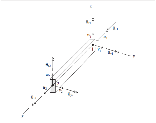
Figure 1: Beam element coordinate system and 12 active degrees-of-freedom of the beam finite element
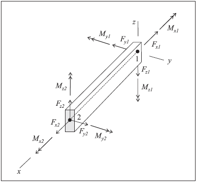
Figure 2: Sign convention for forces and moments at the ends of a beam element (Axes show beam element coordinate system, ends 1 and 2 correspond with order in nodal connectivity list, and all quantities are drawn acting in their positive sense.)
The beam element coordinate system can be modified with the structure beam property direction-y command. (If \(\bf Y\) is not specified, or is parallel with the local \(x\)-axis, then \(\bf Y\) defaults to the global \(y\)- or \(x\)-direction, whichever is not parallel with the local \(x\)-axis.) The beam element coordinate system can be viewed with the Beam plot item and printed with the structure beam list system-local command. The nodal connectivity can be printed with the structure beam list information command.
The 12 active degrees-of-freedom of the beam finite element are shown in Figure 1. For each generalized displacement (translation and rotation) shown in the figure, there is a corresponding generalized force (force and moment). The stiffness matrix of the beam finite element includes all six degrees of freedom at each node to represent axial, shear and bending action within a beam structure.
Response Quantities
Beam responses include force and moment vectors that act at the end of each beam element. These quantities can be expressed in the global system or in the beam element coordinate system. The beam responses can be accessed via FISH and
- printed with the
structure beam listcommand, using the subsequent keywords force-node or force-end, - monitored with the
structure beam historycommand, and - visualized with the Beam plot item.
The sign convention in Figure 2 provides a continuous description of force and moment distributions across beam elements that make up a single beam. It assumes that the set of beam elements making up the beam are oriented consistently, such that their local coordinate systems form a continuous description of the beam orientation. Such will be the case if the beam is created using the structure beam create command. The nodes of each beam element so created will be ordered such that the overall beam direction goes from the first point to the second point specified. The nodal connectivity can be printed with the structure beam list information command.
Properties
Each beam element has 12 properties:
- density, mass density, \(\rho\) (optional — needed if dynamic mode or gravity is active) [M/L3]
- young, Young’s modulus, \(E\) [F/L2]
- poisson, Poisson’s ratio, \(\nu\)
- plastic-moment, plastic moment capacity in Y and Z , \(M^P\) (optional — if not specified; \(M^P\) is assumed to be infinite) [F\(\cdot\)L] If plastic moment was specified in Y and Z directions separately then this value is the maximum of those components. If assigned the value is given to both the y and z components.
- plastic-moment-y, plastic moment capacity in Y only, \(M^P\) (optional — if not specified; \(M^P\) is assumed to be infinite) [F\(\cdot\)L]
- plastic-moment-z, plastic moment capacity in Z only, \(M^P\) (optional — if not specified; \(M^P\) is assumed to be infinite) [F\(\cdot\)L]
- thermal-expansion, thermal expansion coefficient , \(\alpha_t [1/T]\) (optional — used for thermal analysis)
- cross-sectional-area, cross-sectional area, \(A\) [L2]
- moi-y, second moment with respect to beam element \(y\)-axis; \(I_y\) [L4]
- moi-z, second moment with respect to beam element \(z\)-axis; \(I_z\) [L4]
- moi-polar, polar moment of inertia, \(J\) [L4]
- direction-y, vector \(\bf Y\) whose projection onto the beam element cross-section defines the element \(y\)-axis (optional — if not specified, \(\bf Y\) defaults to the global \(y\)- or \(x\)-direction, whichever is not parallel with the element \(x\)-axis)
The material behavior is described by properties 1-5, and the cross-sectional geometry is described by properties 6-10. For the general beam element cross-section shown in Figure 3, the polar moment of inertia, \(J\), and second moments, \(I_y\) and \(I_z\), are defined in the element coordinate system \(xyz\) by the integrals
in which the two principal axes of the cross section are defined by the beam element \(y\)- and \(z\)-axes.
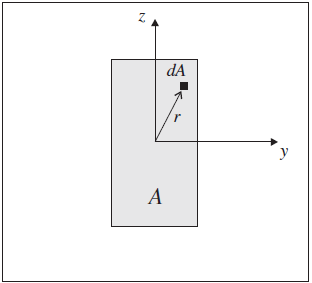
Figure 3: General beam element cross-section in the element yz-plane
Beam properties are easily calculated, or obtained from handbooks. For example, typical values for structural steel are 200 GPa for Young’s modulus, and 0.3 for Poisson’s ratio. For concrete, typical values are 25 to 35 GPa for Young’s modulus, 0.15 to 0.2 for Poisson’s ratio, and 2100 to 2400 kg/m3 for mass density. Composite systems, such as reinforced concrete, should be based on the transformed section.
If a plastic moment is specified, the value may be calculated as follows. Consider a flexural member of width, \(b\), and height, \(h\). If the member is composed of a material that behaves in an elastic-perfectly plastic manner, the elastic and plastic resisting moments can be computed. The moment necessary to produce yield stress, \(\sigma_y\), in the outer fibers is defined as the elastic moment, \(M^E\), and is calculated as
For yielding to occur throughout the section, the yield stress must act on the entire section, and the location of the resultant force on one-half of the section must be \(h/4\) from the neutral surface. The resisting moment, defined as the plastic moment, \(M^P\), is
The section at which the plastic moment occurs can continue to deform without inducing additional resistance after it reaches \(M^P\). The plastic-moment capacity limits the internal moment carried by each beam element.
In order to limit the moment that is transmitted between beam elements, the moment capacity at the nodes must also be restricted. The condition of increasing deformation with a limiting resisting moment that results in a discontinuity in the rotational motion is called a plastic hinge. Potential plastic-hinge locations can be defined by creating double nodes at each hinge location, adding a node-to-node link between these nodes, and then specifying appropriate link attachment conditions. If the limiting moment is reached at beam element connected by such a plastic hinge double-node, then a discontinuity in the rotational motion will develop. See Plastic Hinge Formation in a Beam Structure for an example application of plastic hinges modeled with both single and double nodes.
The preceding discussion assumes a section that is symmetric about the neutral axis. However, if the section is not symmetric (for example, a T-section), or if the stress-strain relations for tension and compression differ appreciably (for example, reinforced concrete), the neutral axis shifts away from the fibers that yield first, and it is necessary to relocate the neutral axis before the resisting moment can be evaluated. The neutral axis may be found by integrating the stress profile over the section and solving for the location of the axis at which stress is zero. In some cases, the integral can be expressed in terms of one unknown (in which case, the solution may not be difficult). However, if the stress-strain relation for the material does not resemble an ideal elasto-plastic diagram, the solution may involve a number of trials. Nearly all texts on reinforced concrete or steel design provide procedures and examples for calculating plastic moments.
The present formulation in the program assumes that beam elements behave elastically until they reach the plastic moment. This assumption is reasonably valid for symmetric rolled-steel sections, because the difference between \(M^P\) and \(M^E\) is not large. However, for reinforced concrete, the plastic moment may be as much as an order of magnitude greater than the elastic moment.
Example Applications
Simple examples are given to illustrate the use of beams.
A complete list of examples that use beam elements is available in Structural Beam Examples.
Commands & FISH
| Was this helpful? ... | 3DEC © 2019, Itasca | Updated: Feb 25, 2024 |