Dewatered Construction of a Braced Excavation
Problem Statement
Note
The project file for this example is available to be viewed/run in FLAC3D.[1] The project’s main data file is shown at the end of this example.
A braced excavation is constructed in saturated ground. The excavation is dewatered during construction and is supported by diaphragm walls that are braced at the top by horizontal struts. The purpose of the FLAC3D analysis is to evaluate: 1) the deformation of the ground adjacent to the walls and at the bottom of the excavation; and 2) the performance of the walls and struts throughout the construction stages. The analysis starts from the stage after the walls have been constructed, but prior to any excavation. Dewatering, excavation, and installation of struts are simulated in separate construction stages. In addition, three different material models, the Mohr-Coulomb model, the CYSoil model, and the PH model (without and with small-strain stiffness option) are used to represent the behavior of the soils and demonstrate the difference in deformational response produced by these models when subjected to this construction sequence.
In practice, the construction may involve several stages of dewatering, excavation, and adding of support. For simplicity, in this example, only three construction stages are analyzed: 1) dewatering to a 20 m depth in the region to be excavated; 2) excavation to a 2 m depth; and 3) installation of a horizontal strut and excavation to a 10 m depth. Additional excavation stages can readily be incorporated in the FLAC3D analysis, as required.
Figure 1 shows the geometry for this example, along with names assigned in two different groups by the Extruder tool. The top set of names in the “Construction” slot was assigned interactively, while the second set of names in the “Block” slot was assigned automatically by the Extruder. The excavation is 20 m wide and the final depth is 10 m. The diaphragm walls extend to a 30 m depth and are braced at the top by horizontal struts at a 2 m interval. The ground consists of two soil layers: a 20 m thick soft clay underlain by a stiff sand layer that extends to a great depth. The initial water table is at the ground surface.
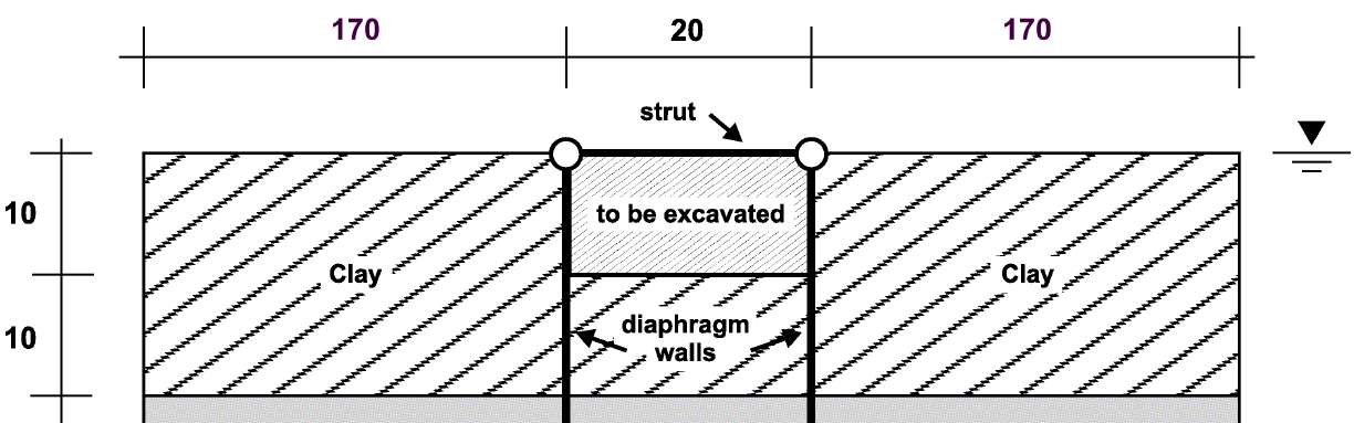
Figure 1: Geometry for braced excavation example.
The properties selected to simulate the behavior of the diaphragm wall and the struts in this example are listed in Table 1 and Table 2. The thickness of the diaphragm wall varies, and an equivalent thickness is estimated to be 1.26 m.
The strut properties are listed in Table 2. The spacing of the struts is 2 m.
The hydraulic conductivity of the soils is assumed to be a constant value of 10-6 m/sec (which corresponds to approximately 10-10 m2/(Pa-sec) for the mobility coefficient).
| Equivalent thickness (m) | 1.26 |
| Density (kg/m3) | 2000 |
| Young’s modulus (GPa) | 5.712 |
| Poisson’s ratio | 0.2 |
| Moment of inertia (m4) | 0.167 |
| Cross-sectional area (m2) | 1.0 |
| Spacing (m) | 2.0 |
| Density (kg/m3) | 3000 |
| Young’s modulus (GPa) | 4.0 |
| Moment of inertia (m4) | 0.083 |
Problem Statement
The deformation of the soils during excavation is of particular interest in this example, specifically the heave at the bottom of the excavation and the surface settlement adjacent to the excavation wall. Two different material models, the Mohr-Coulomb model and the CYSoil model, are used to illustrate the effect of the material model on the calculated deformational response of the soil. It is noted that for uniform elastic properties, the linear elastic/perfectly plastic Mohr-Coulomb model may predict unrealistically large deformations in soils subjected to loading and unloading, such as heave induced at the bottom of excavations. A more realistic calculation may be obtained with the nonlinear elastic/plastic CYSoil model.
The drained material properties for the Mohr-Coulomb Model associated with the sand and clay are summarized in Table 3.
The PH model properties are listed in Table 4.
The formulation of the CYSoil model has components in common with the PH model. A connection, as shown in Table 5, is proposed between hardening CYSoil properties and PH properties. Note, however, that among other things, differences exist in the hardening and dilatancy laws. (See the PH model for a description.) Thus, the model responses should not be expected to be identical.
| Sand layer | Clay layer | |
|---|---|---|
| Dry density (kg/m3) | 1700 | 1600 |
| Young’s modulus (MPa) | 40.0 | 10.0 |
| Poisson’s ratio | 0.30 | 0.35 |
| Cohesion (MPa) | 0 | 0 |
| Friction angle (degrees) | 32 | 25 |
| Dilation angle (degrees) | 2 | 0 |
| Porosity | 0.3 | 0.3 |
| PH Model Property | Sand layer | Clay layer |
|---|---|---|
| Dry density (kg/m3) | 1700 | 1600 |
| \(p_{ref}\) (kPa) | 100 | 100 |
| \(E^{ref}_{50}\) (MPa) | 30 | 8 |
| \(E^{ref}_{ur}\) (MPa) | 90 | 24 |
| \(E^{ref}_{oed}\) (MPa) | 30 | 4 |
| Poisson’s ratio, \(\nu_{ur}\) | 0.2 | 0.2 |
| Cohesion (kPa) | 1 | 5 |
| Friction angle (degrees) | 32 | 25 |
| Dilation angle (degrees) | 2 | 0 |
| Power, \(m\) | 0.5 | 0.8 |
| \(K^{nc}_{0}\) | 0.47 | 0.50 |
| Failure ratio, \(R_f\) | 0.9 | 0.9 |
| PH Model | CYSoil Model |
|---|---|
| \(E^{ref}_{50}\) | – |
| \(E^{ref}_{ur}\) | \(G_{ref} = {E^{ref}_{ur} \over p_{ref}} \cdot {(1-2\nu) \over {2(1-2\nu)}}\) |
| \(E^{ref}_{oed}\) | \(R = {E^{ref}_{ur} \over E^{ref}_{oed}} \cdot {{1-\nu} \over {(1+\nu)(1-2\nu)}} - 1\) |
| Friction angle, \(\phi\) | \(\phi_f\) |
| Dilation angle, \(\psi\) | \(\psi_f\) |
| Poisson’s ratio, \(\nu\) | \(\nu\) |
| Exponent, \(m\) | \(m\) |
| Failure ratio, \(R_f\) | \(R_f\) |
The following procedure is used to develop properties for the CYSoil model in this example. The CYSoil model can represent the nonlinear stress/strain response for loading and unloading that is characteristic of soils.
Table 5 is used to derive the hardening CYSoil properties shown in Table 6. The FISH function setup performs the derivation of CYSoil properties from the Hardening Soil properties. Note that the cap-yield surface parameter, \(\alpha\), is set to one. [4]
The soils are assumed to be normally consolidated. Accordingly, initial (mobilized) friction is calculated from the initial stress using the equation
\[\sin \phi_m = {{\sigma'_1 - \sigma'_3} \over {\sigma'_1 + \sigma'_3 - 2c \cot \phi_f}}\]which is calculated in FISH function ini�_cy, listed in “setup.dat”.
Table 6: Hardening CYSoil Properties Sand layer Clay layer Dry density, \(\rho\) (kg/m3) 1700 1600 Cap-yield surface parameter, \(\alpha\) 1.0 1.0 Ultimate friction angle, \(\phi_f\) (degrees) 32 25 Ultimate dilation angle, \(\psi_f\) (degrees) 2 0 Multiplier, \(R\) 2.333 5.667 \(G_{ref}\) 112.5 15.0 Reference pressure, \(p_{ref}\) (kPa) 100 100 Poisson’s ratio, \(\nu_{ur}\) 0.2 0.2 Cohesion (kPa) 1 5 Power, \(m\) 0.5 0.8 \(K^{nc}_0\) 0.47 0.50 Initial mobilized friction angle, \(\phi_m\) (degrees) 19.47 19.47 Failure ratio, \(R_f\) 0.9 0.9 The CYSoil properties \(K^e\) and \(G^e\) are stress-dependent, and these properties are specified after the initial pre-excavation stress state is established. The commands
zone waterandzone initialize-stressesare used to initialize pore pressures and stresses automatically from the known \(K_0\) and for the initial water level at the ground surface.The CYSoil property \(p_c\) is also stress-dependent. It is assumed that the clay and sand are normally consolidated on the cap (ocr = 1), so that \(p_c\) = \(p_{ini}\). The initial effective stress is used to calculate the initial values for \(p^{\prime}\) and \(q\). The cap and initial pressure is assigned in FISH function ini�_cy, listed in “setup.dat”.
The PH properties \(\sigma^{ini}_1\), \(\sigma^{ini}_2\) and \(\sigma^{ini}_3\) are stress-dependent. These effective principal stresses are initialized in FISH function ini�_ph, listed in “setup.dat”.
The input parameter flag-cap = 1 indicates that the cap is activated.
The default parameter flag-dilation (0) implies that the built-in Rowe rule is used; the default parameter flag-shear (0) implies that the built-in shear hardening law is used. All the formula are described in the CYSoil model.
Modeling Procedure
A recommended procedure to simulate this type of problem with FLAC3D is illustrated by performing the analysis in six steps.
Step 1: Generate the model grid and assign material models, material properties, and boundary conditions to represent the physical system. Step 2: Determine the initial in-situ stress state of the ground prior to construction. Step 3: Determine the initial in-situ stress state of the ground with the diaphragm wall installed. Step 4: Lower the water level within the region to be excavated to a depth of 20 m below the ground surface. Step 5: Excavate to a depth of 2 m. Step 6: Install the horizontal struts at the top of the wall, and then excavate to a depth of 10 m.
Three data files were created for the above steps: for the Mohr-Coulomb model, the CYSoil model and PH model, respectively. The Mohr-Coulomb data file is named “BracedExcavation-mc.dat”. The CYSoil data file is named “BracedExcavation-cy.dat”. The PH material without small-strain stiffness data file is named “BracedExcavation-ph.dat”. The PH with small-strain stiffness data file is named “BracedExcavation-phss.dat”. Listings of these files are provided in the data files. The only difference between the PH material with small-strain stiffness and the PH material without small-strain stiffness is one line that turns on the small-strain flag:
zone property flag-smallstrain on
Model Generation
It is only necessary to consider half of the problem region shown in Figure 1 because of the symmetric geometry. This grid is created interactively using the Extruder tool, which is also used to name regions of the model for later reference. Zoning near the excavation is a uniform 1 m, with the zone size gradually increasing farther away from the excavation. The grid is initially divided into four groups names, “clay-left”, “clay-right”, “sand-left”, and “sand-right”, which correspond to zones on the left and right sides of the diaphragm wall and the sand and clay layers. The face group “Liner” is assigned between the “left” and “right” sides at the correct elevation. The embedded liner is then installed at the face group “Liner”:
struct liner create by-face separate cross-diagonal range group 'Liner'
The embedded liner has independent properties on each side of the liner. Although the properties can be different, in this example they are the same on each side. Normal and shear coupling springs are used to interface the embedded liner to the zones.
It is usually reasonable to select the interface normal and shear stiffness properties such that the stiffness is approximately ten times the equivalent stiffness of the stiffest neighboring zone. By doing this, the deformability at the interface will have minimal influence of both the compliance of the total model and the calculation speed. The equivalent stiffness of a zone normal to the interface is
where \(K\) and \(G\) are the bulk and shear moduli, respectively, and \(\Delta z_{\min}\) is the smallest width of an adjoining zone in the normal direction. The \(\max\) [ ] notation indicates that the maximum value over all zones adjacent to the interface is to be used (e.g., there may be several materials adjoining the interface).
In this example, the smallest grid width adjacent to the interface is 1 m and the maximum equivalent stiffness is approximately 55 MPa. Therefore, a representative value of 550 MPa/m is selected for the normal and shear stiffnesses.
The density of the wall is not assigned at this stage, because first the equilibrium stress state will be calculated before the wall is constructed. This is done by neglecting the weight of the wall.
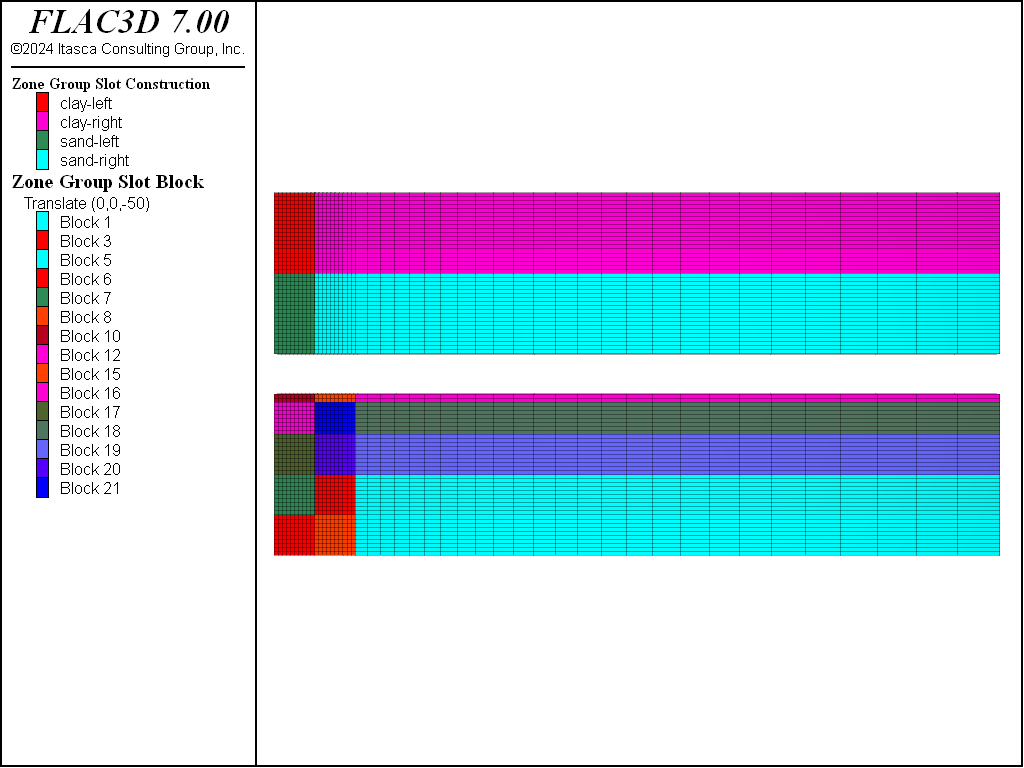
Figure 2: Grid created for braced excavation.
The groundwater properties porosity and permeability are assigned. Note that the “permeability” required by FLAC3D is actually the mobility coefficient (i.e., the coefficient of the pore pressure term in Darcy’s law—see Fluid Permeability Coefficient). Gravity is set to 10.0 m/sec2 to simplify this example. Set the water density to 1000 kg/m3. Roller boundaries are placed on the left, right, front, and rear boundaries of the grid. The bottom of the grid is fixed.
Before saving the initial state, the static equilibrium is specified for the initial pre-excavation
stress state with the water table at the ground surface. The pore pressure and total (and
effective) stress distributions must be compatible at the initial state. The pore pressures are
assigned using the zone water command and a uniform horizontal plane at an elevation of 40.
The initial stresses are assigned using the command zone initialize-stresses using a
\(K_0\) ratio of 0.47 in the sand and 0.50 in the clay. After the pore pressure distribution is calculated, fix the pore pressures
along the top and side boundaries, and saturation along the top boundary to satisfy the flow
conditions. The initial pore-pressure distribution is shown in Figure 3.
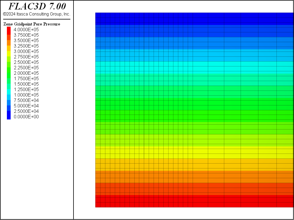
Figure 3: Initial pore-pressure distribution.
The above steps are common to the Mohr-Coulomb, CYSoil and PH examples. The CYSoil and PH model requires additional setup. With the CYSoil and PH model, it is necessary to specify the stress-dependent properties and hardening table functions if required. These are applied as FISH functions, as described in “BracedExcavation-cy.dat”. The FISH function setup is executed first to derive CYSoil-related properties based on Hardening Soil properties. The stress-dependent properties for the CYSoil mdoel are input in the FISH function ini�_cy. Similarly, the stress-dependent properties for the PH model are input in the FISH function ini�_ph.
Initial Conditions
A check is made to verify that the models are in equilibrium with the prescribed initial and
boundary conditions. While the liner interface springs are initialized using the
structure liner initialize coupling command, a slight stress readjustment is still made near
the diaphragm wall.
Install Diaphragm Wall
The next stage of the analysis is the installation of the diaphragm wall. This is simulated by assigning the wall its proper weight by specifying a density for the embedded liner. Also, turn off the flow mode and ensure that the water bulk modulus is zero because the generation of pore pressures is not desired during this stage. The three models are solved and saved in “mc-part-3”, “cy-part-3”, and “ph-part-3”.
Figure 4, Figure 5, Figure 6, and Figure 7 show the total vertical stress distribution for the Mohr-Coulomb, CYSoil and PH models at this stage. There is a slight difference in stress distribution around the wall in the CYSoil material compared to the wall in Mohr-Coulomb material. This can be attributed to the difference between the stress-dependent stiffness properties of the CYSoil material and the constant, uniform stiffness properties of the interfaces adjacent to the wall. Although the difference is minor, a stress-dependent variation of interface stiffnesses could be applied using FISH in order to provide a closer representation.
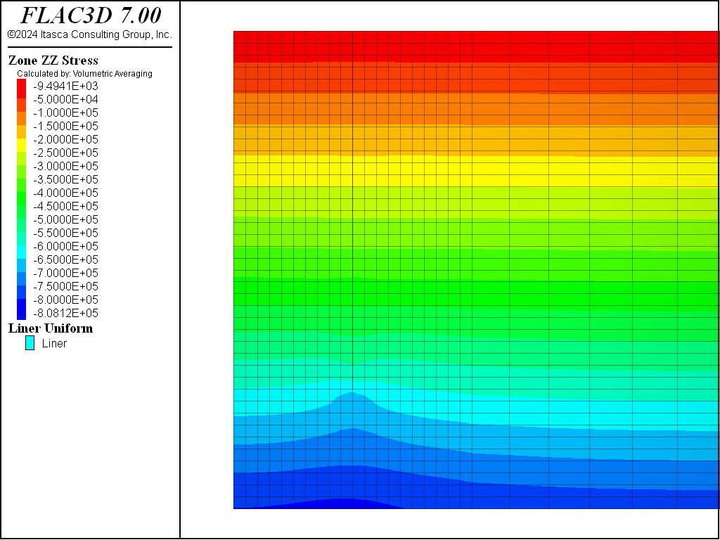
Figure 4: Total vertical stress contours for initial saturated state with weight of wall included—Mohr-Coulomb material.
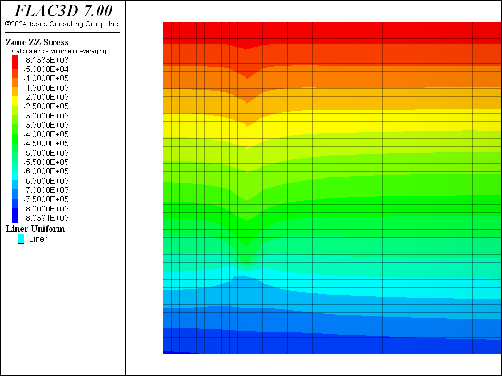
Figure 5: Total vertical stress contours for initial saturated state with weight of wall included—CYSoil material.
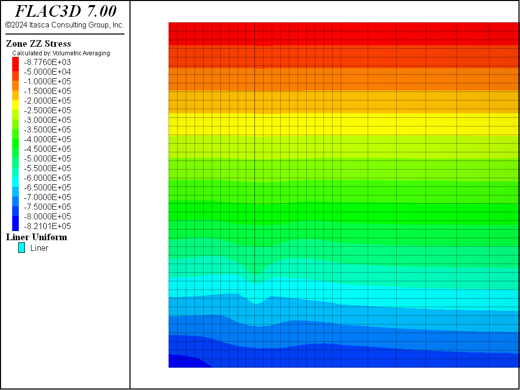
Figure 6: Total vertical stress contours for initial saturated state with weight of wall included—PH material.

Figure 7: Total vertical stress contours for initial saturated state with weight of wall included—PH material with small-strain stiffness.
Dewater to a Depth of 20 m
For the dewatering stage, assume for simplicity that the water level is dropped instantaneously within the excavation region [5]. Start from the previous step and set the saturation, pore pressure, and permeability to zero in the excavation area (all zones belonging to group “clay-left”). Free the fixed pore-pressure condition along the left boundary below the excavation and along the top of the model to the right of the excavation so that pore pressures can change during dewatering. Initialize the displacements in the model to zero so that the displacement change that occurs due only to the dewatering can be monitored.
When a change in pore pressure is imposed, the total stress must be adjusted to account for this
change. This is done using the zone gridpoint fix pore-pressure 0 command.
When this command is used to modify existing pore-pressures, the change is stored and applied to
the total stress state in the next step. In this way, the total stresses are adjusted, but the
effective stresses remain the same. Note that if the zone gridpoint initialize pore-pressure
command was used, the total stresses would remain the same but the effective stresses would be
adjusted.
Check that this adjustment to total stress has been made by plotting effective stresses before and after these commands are issued as long as at least one step is taken: the effective stresses are unchanged in the model when the instantaneous pore pressure is imposed.
Now solve for the coupled response that results from the dewatering. Groundwater flow is set on, and the water bulk modulus is set to 10,000 Pa. The water bulk modulus needs to be specified for this calculation, so this low value is specified in order to speed convergence to steady-state flow. This can be done because the transient behavior is not of interest. (Note that there is a lower limit for the water bulk modulus to satisfy numerical stability — see Fluid Time Scales.)
For the Mohr-Coulomb material, the steady-state pore-pressure distribution after dewatering is shown in Figure 8. Figure 9 plots the displacement vectors at equilibrium. This indicates the amount of settlement induced by the dewatering, approximately 15 cm. The model state is saved as as “mc-part-4” for the Mohr-Coulomb material.
This dewatering procedure is repeated for the CYSoil material. The final pore-pressure distribution is shown in Figure 10 and is nearly identical to that for the Mohr-Coulomb material, as shown in Figure 8. The displacements induced by dewatering are shown in Figure 11. The model with CYSoil material is saved at this stage as “cy-part-4”.
This dewatering procedure is again repeated for the PH material. The final pore-pressure distribution is shown in Figure 12 and displacements induced by dewatering are shown in Figure 13. The model with PH material is saved at this stage as “ph-part-4”.
This dewatering procedure is again repeated for the PH material with small-strain stiffness option. The final pore-pressure distribution is shown in Figure 14 and displacements induced by dewatering are shown in Figure 15. The model with PH material with small-strain stiffness option is saved at this stage as “phss-part-4”.

Figure 8: Pore pressure distribution following dewatering—Mohr-Coulomb material.
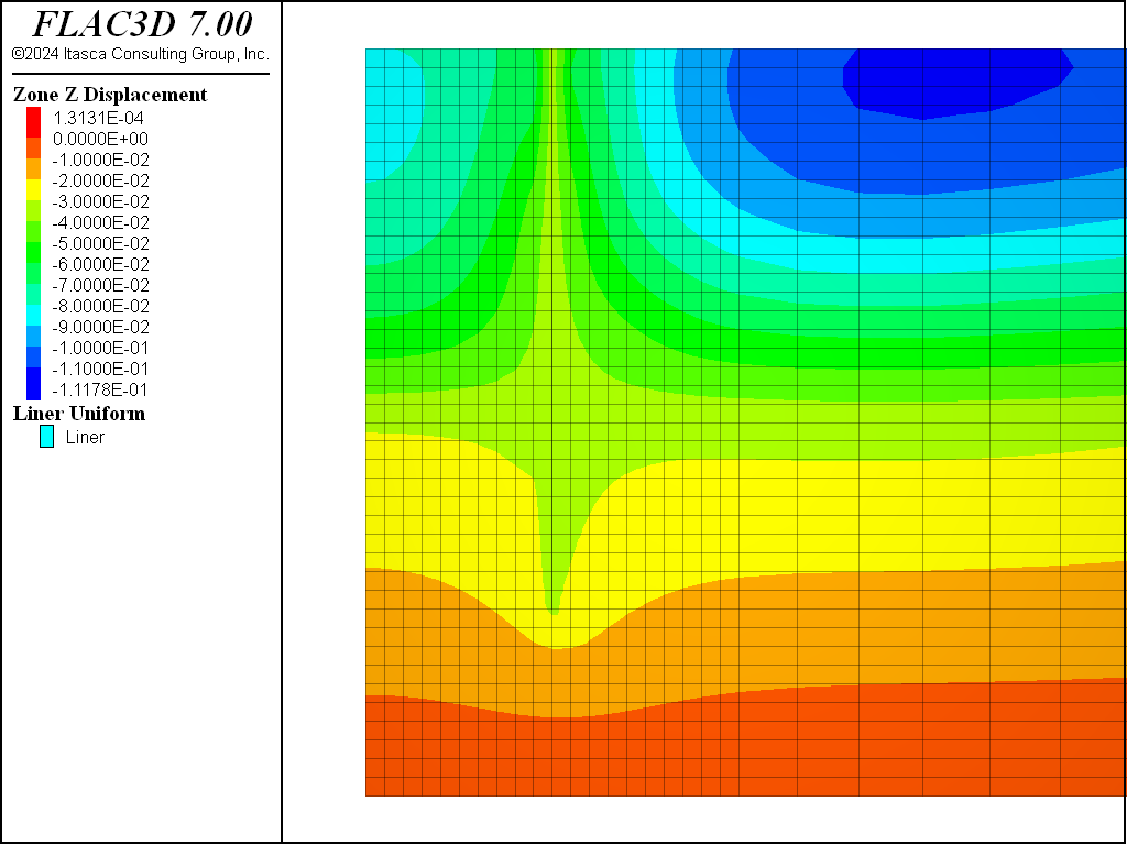
Figure 9: Displacements induced by dewatering—Mohr-Coulomb material.

Figure 10: Pore pressure distribution following dewatering—CYSoil material.
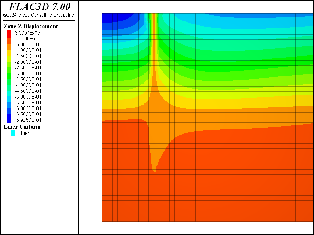
Figure 11: Displacements induced by dewatering—CYSoil material.

Figure 12: Pore pressure distribution following dewatering—PH material.
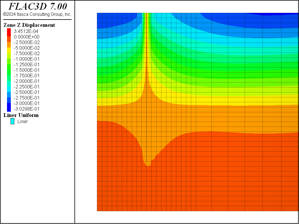
Figure 13: Displacements induced by dewatering—PH material.
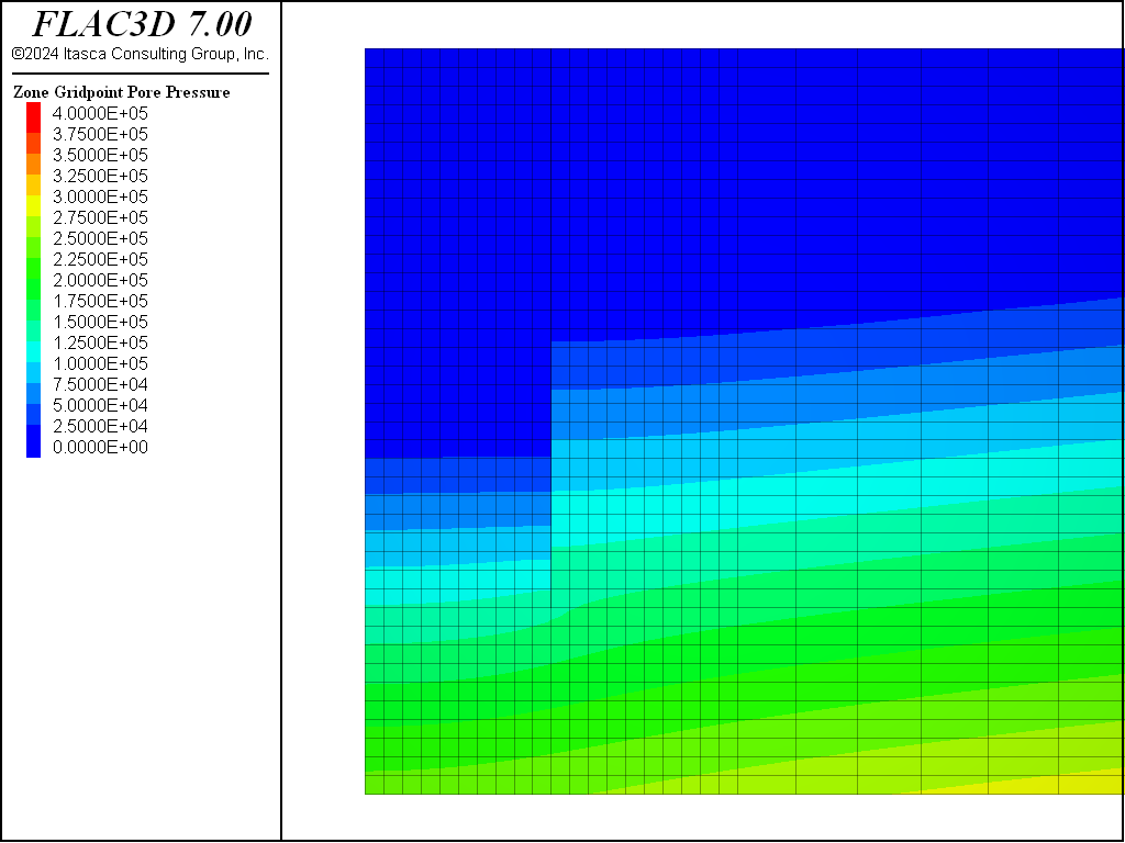
Figure 14: Pore pressure distribution following dewatering—PH material with small-strain stiffness option.
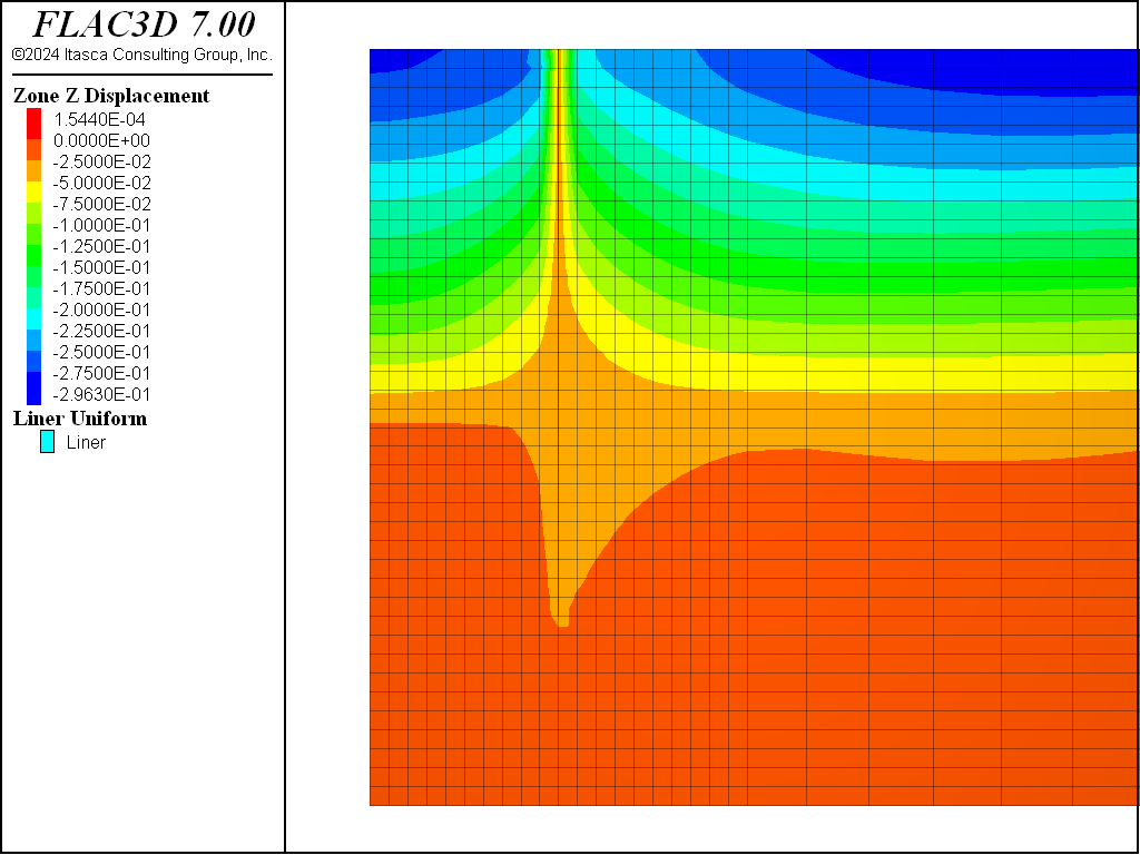
Figure 15: Displacements induced by dewatering—PH material with small-strain stiffness option.
Excavate to 2 m Depth
The excavation to 2 m can now begin. Start from “mc-part-4”, “cy-part-4”, “ph-part-4”, and “phss-part-4”, set flow off, and set the water bulk modulus to zero for this mechanical-only calculation. The displacements are initialized to zero in order to evaluate the deformation induced by the excavation.
Excavate by deleting zones in the range of the material to be removed (using the command zone delete), using the block name assigned by the Extruder tool. (A null model could be assigned to these zones, but these zones will no longer be required for the remainder of the modeling.) Figure 16 or Figure 17 shows a close-up of a portion of the grid with the 2 m excavation.
At this point, the model is solved. This is the long-term response (with the water bulk modulus set to zero). The models are saved as “mc-part-5”, “cy-part-5”, “ph-part-5”, and “phss-part-5”.
The displacements induced by this excavation are illustrated in Figure 16, Figure 17, Figure 18, and Figure 19 for the Mohr-Coulomb, CYSoil and PH models (without and with small-strain stiffness, respectively). With the Mohr-Coulomb model, a maximum heave of roughly 3.4 cm occurs at the bottom of the excavation. With the CYSoil model, a maximum heave of roughly 1.6 cm occurs at the bottom of the excavation. With the PH model without small-strain stiffness, a maximum heave of roughly 2.7 cm occurs at the bottom of the excavation. For the PH model with small-strain stiffness, the maximum heave is only 1.6 cm.
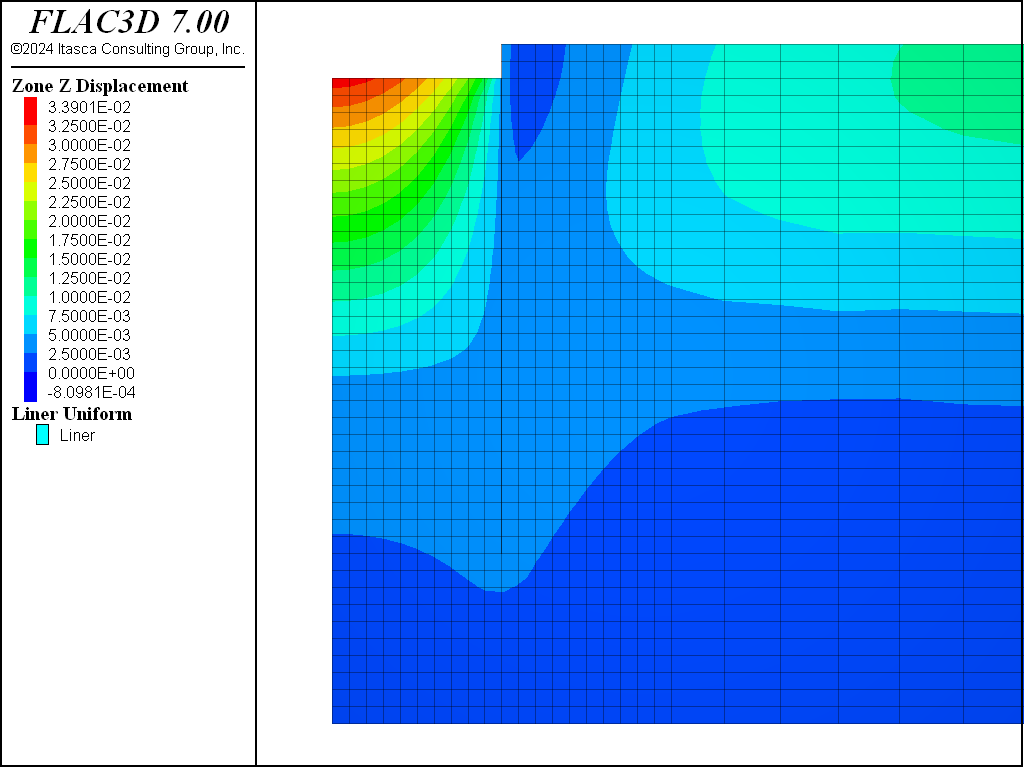
Figure 16: Displacements induced by excavation to 2 m depth—Mohr-Coulomb material.
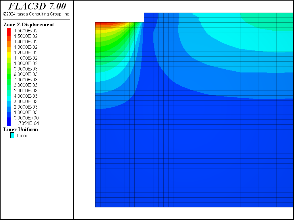
Figure 17: Displacements induced by excavation to 2 m depth—CYSoil material.
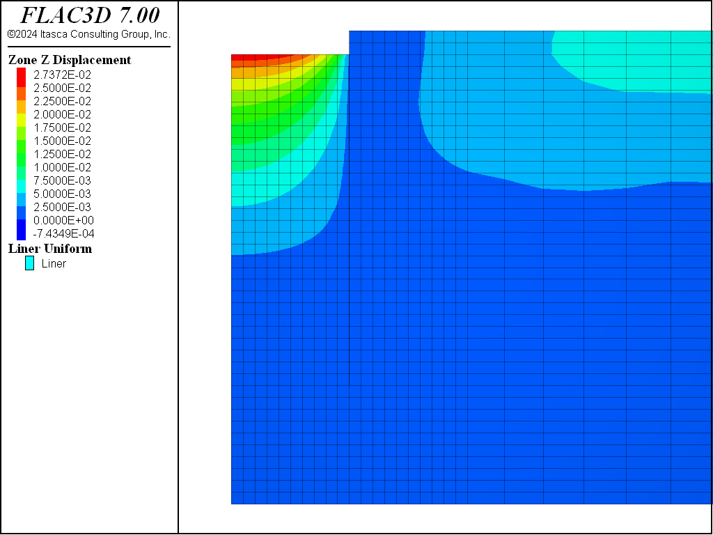
Figure 18: Displacements induced by excavation to 2 m depth—PH material.
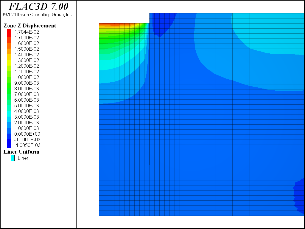
Figure 19: Displacements induced by excavation to 2 m depth—PH material with small-strain stiffness.
The response of the wall can also be calculated. For example, the moment distribution in the wall after the first excavation is shown in Figure 20. Note that the various results for the wall response (e.g., wall displacements, shear forces) can be plotted using the Liner plot item in FLAC3D.
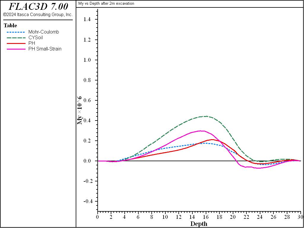
Figure 20: Bending stress resultant \(M_y\) in wall after excavation to 2 m depth—Mohr-Coulomb and CYSoil material.
Install Strut and Excavate to 10 m Depth
For the final excavation step, install a horizontal strut at the top of the wall and then excavate to a 10 m depth. The strut is not rigidly connected to the wall in this exercise. A pin connection is defined (which permits free rotation at the strut/wall connection). The strut consists of a single beam element at an elevation equal to the ground elevation before excavation, extending from the symmetry plane (\(x = 0\) plane) to a point on the diaphragm wall ((\(x,y,z\)) = (10,1,40)).
First the horizontal strut is created, making certain the end connects to a liner node, and material properties are assigned with the commands
struct beam create by-line (0,1,40) (10,1,40) snap group 'Beam'
struct beam property density 3000.0 young 4.0E9 poisson 0.30 ...
                  cross-sectional-area 1.0 moi-y 0.083 moi-z 0.083 ...
                  moi-polar 0.0 range group 'Beam'
For the beam node on the plane of symmetry, all degrees of freedom are fixed, except for the \(z\)-displacement degree-of-freedom, with the command
struct node fix velocity-x velocity-y rotation range group 'Beam' position-x 0
This has the effect of restricting the beam so that it only moves in the vertical direction; rotations \(x\)- and \(y\)-displacements are inhibited.
Next, the beam is joined to the liner with the command
struct node join range group 'Beam'
This command finds nodes residing at the same physical location and links them together.
The rotational degrees-of-freedom at this link are freed with the commands
struct link attach rotation-x free rotation-y free rotation-z free ...
                   range group 'Beam' position-x 10
The second excavation step is performed by deleting zones within the second excavated region with the command
zone delete range group 'Block 15'
At this point, all zones from the surface (\(z\) = 40 m) to the bottom of the clay-1 layer (\(z\) = 10 m) are deleted and we are ready to solve. After reaching equilibrium, the state is saved in file “mc-part-6” (for the Mohr-Coulomb case), file “cy-part-6” (for the CYSoil case), and file “ph-part-6” (for the PH case).
The total displacements induced by the excavation to the 10 m depth of these three cases are illustrated in Figure 21, Figure 22, Figure 23, and Figure 24, respectively.
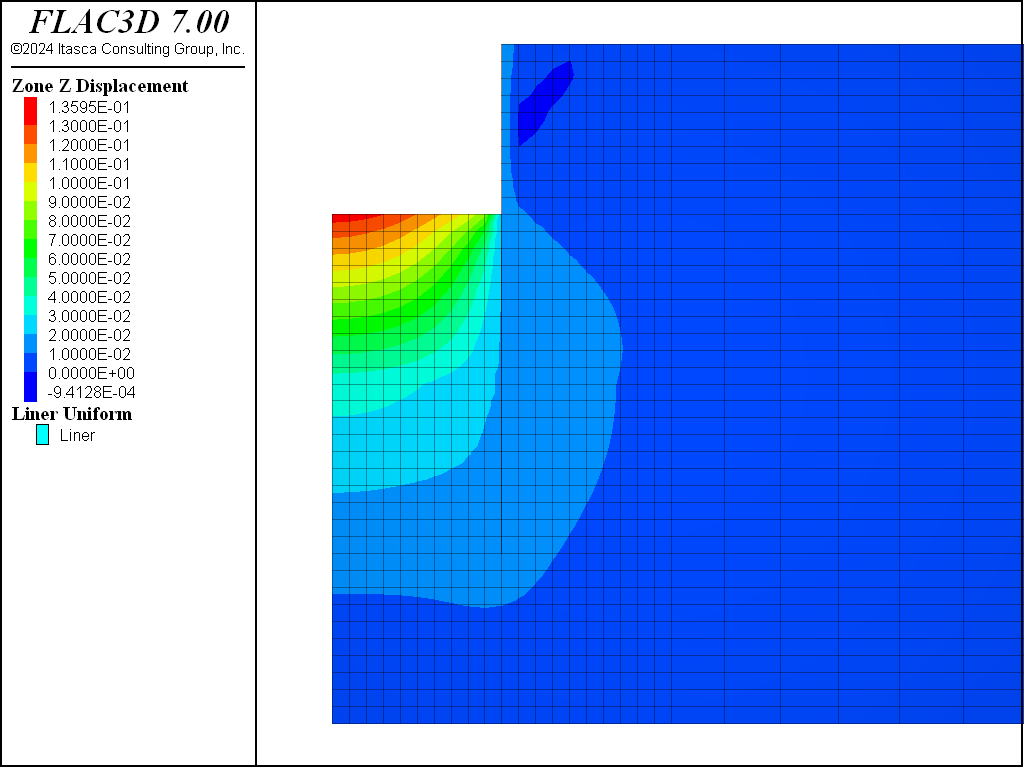
Figure 21: Displacements induced by excavation to 10 m depth—Mohr-Coulomb material.
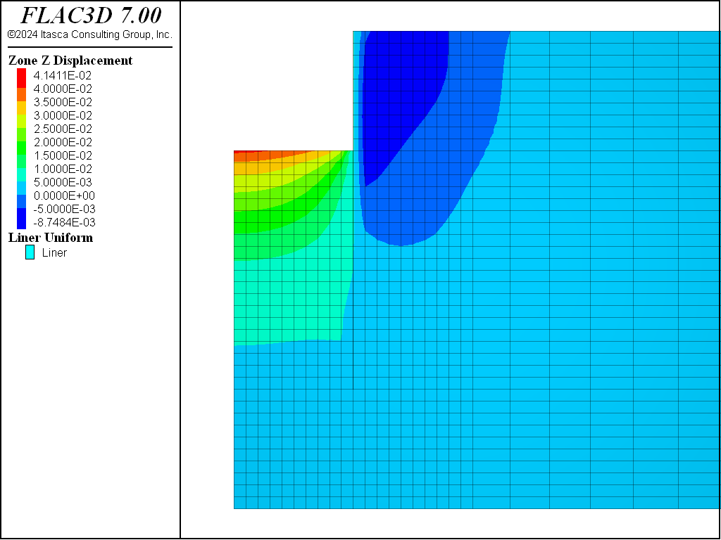
Figure 22: Displacements induced by excavation to 10 m depth—CYSoil material.
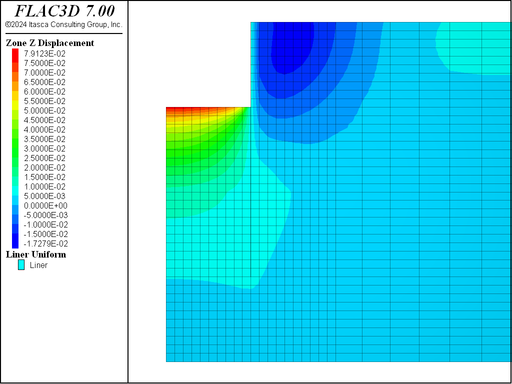
Figure 23: Displacements induced by excavation to 10 m depth—PH material.
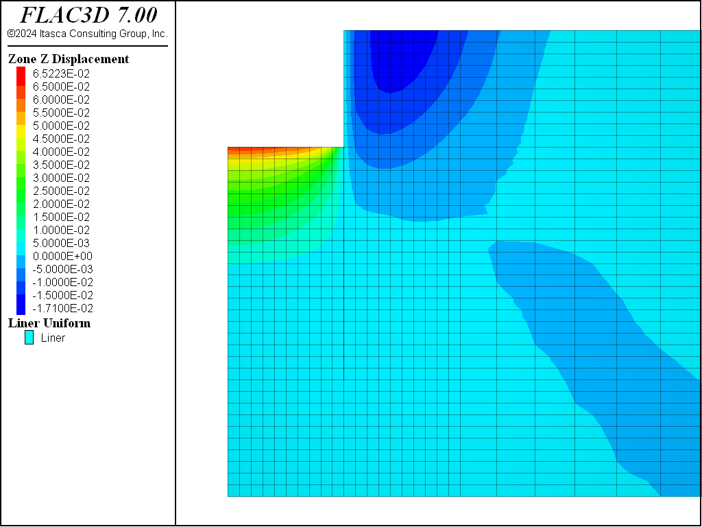
Figure 24: Displacements induced by excavation to 10 m depth—PH material with small-strain stiffness.
Comparing Figure 21, Figure 22, Figure 23, and Figure 24, it can be seen that the maximum displacements for the CYSoil and PH material are much less than for the Mohr-Coulomb material. Also, the extent of the excavation-induced displacement in the CYSoil and PH material is more confined than that for the Mohr-Coulomb material.
The moment distribution in the wall after the second excavation is shown in Figure 25. The maximum momenta are roughly the same for all models.
Figure 26 plots the ground displacement behind the wall. The Mohr-Coulomb material predicts unrealistic negative settlement (upward displacement) at the ground immediately behind the wall, while the CYSoil and PH materials correctly predict positive settlement (downward displacement), but the settlement predicted by CYSoil material is approximately half that of the PH materials. The PH materials without and with small-strain stiffness predict almost the same settlement immediately behind the wall, but the PH material with small-strain stiffness predicts much less upward displacement at the ground far from the wall, which is generally closer to field observations.
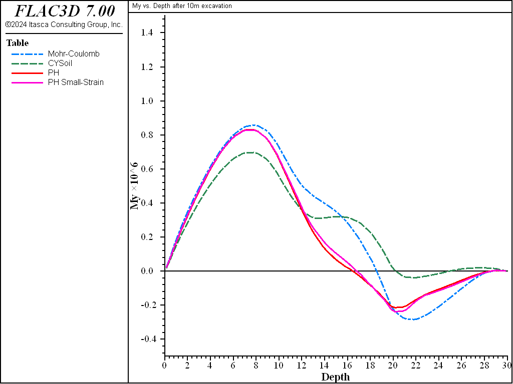
Figure 25: Bending stress resultant \(M_y\) in wall after excavation to 10 m depth—Mohr-Coulomb and CYSoil material.
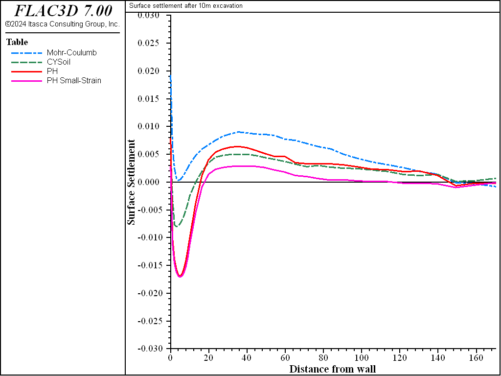
Figure 26: Surface settlement profiles (\(x = 0\) is at diaphragm wall).
Observations
This example illustrates the effect of the material model on soil deformational response for unloading problems such as the construction on a braced excavation. The heave that occurs at the bottom of the excavation is considerably greater for the construction in Mohr-Coulomb material than it is for CYSoil and PH material. This is primarily attributed to the stress-dependent elastic moduli and stiffer unloading response of the CYSoil and PH material. This is evident from the comparison of the displacement contour plots in Figure 21 for the Mohr-Coulomb material, and Figure 22 for the CYSoil material, or Figure 23 and Figure 24 for the PH material, without and with small-strain stiffness, respectively.
References
Plaxis BV. PLAXIS Version 8, Material Models Manual. R. B. J. Brinkgreve, ed. Delft: Plaxis (2002).
Plaxis BV. PLAXIS Version 8, Tutorial Manual. R. B. J. Brinkgreve, ed. Delft: Plaxis (2002).
Data Files
BracedExcavation-mc.dat
; ---------------------------------------------
; Dewatered Construction of a Braced Excavation
; Mohr-Coulomb model
; ---------------------------------------------
model new
model large-strain off
model title 'Braced excavation - Mohr-Coulomb'
; Model geometry and labels created interactively
; in Extruder and exported from State Pane
; -----------------------------------------------
program call 'geometry' suppress
zone generate from-extruder
; Model setup and initialization
; ------------------------------
; fluid model and properties
model configure fluid
zone fluid cmodel assign isotropic
zone fluid property porosity 0.3 permeability 1.0E-10
zone initialize fluid-density 1000
; mechnical properties
zone cmodel assign mohr-coulomb
zone property density 1700 young 40e6 poisson 0.30 friction 32 ...
              dilation 2 cohesion 1e3 ...
              range group 'sand-left' or 'sand-right'
zone property density 1600 young 10e6 poisson 0.35 friction 25 ...
              dilation 0 cohesion 5e3 ...
              range group 'clay-left' or 'clay-right'
; Create liner and properties
struct liner create by-zone-face separate cross-diagonal range group 'Liner'
struct liner property isotropic (5.712e9, 0.2) thickness 1.26 ...
                      density 0 ; <--- note zero density
struct liner property coupling-stiffness-normal 5.5E9 ...
                      coupling-stiffness-shear 5.5E9 ...
                      coupling-cohesion-shear 2500000.0 ...
                      coupling-friction-shear 12.5 ...
                      coupling-yield-normal 0 ...
                      coupling-cohesion-shear-residual 2500.0
struct liner property coupling-stiffness-normal-2 5.5E9 ...
                      coupling-stiffness-shear-2 5.5E9 ...
                      coupling-cohesion-shear-2 2500000.0 ...
                      coupling-friction-shear-2 12.5 ...
                      coupling-yield-normal-2 0 ...
                      coupling-cohesion-shear-residual-2 2500.0
; initialize stresses and pore pressure
model gravity 10
zone water density 1000
zone water plane origin (0,0,40) normal (0,0,1)
zone initial-stresses ratio 0.47 range group 'sand-left' or 'sand-right'
zone initial-stresses ratio 0.5 range group 'clay-left' or 'clay-right'
struct liner initialize coupling ; initialize liner coupling springs
                                 ; to come to equilibrium faster.
; Boundary conditions - roller on sides, fixed on bottom, fixed pp on top,
; fixed to current values on left and right.
zone face apply velocity-y 0 range group 'Front' or 'Back'
zone face apply velocity-x 0 range group 'Left' or 'Right'
zone face apply velocity (0,0,0) range group 'Bottom'
zone face apply pore-pressure 0 range group 'Top'
zone gridpoint fix pore-pressure range group 'Right'
zone gridpoint fix pore-pressure range group 'Left'
model save 'mc-part-1'
; Come to initial equilibrium -- Without liner we would be in equilibrium,
; with liner we need to adjust
; ------------------------------------------------------------------------
model fluid active off
model mech active on
model solve ratio-local 1e-4
model save 'mc-part-2'
; Activate the liner
; ------------------
zone gridpoint initialize displacement (0,0,0) ; Reset displacements in the
                                               ; model, so we can track
                                               ; incremental changes.
struct liner property density 2000 ; real liner density
zone gridpoint initialize fluid-modulus 0.0
model solve ratio-local 1e-4
model save 'mc-part-3'
; Dewater to a depth of 20m
; -------------------------
zone gridpoint initialize displacement (0,0,0) ; Reset displacements in the
                                               ; model, so we can track
                                               ; incremental changes.
zone gridpoint fix pore-pressure 0.0 range group 'clay-left'
zone gridpoint initial saturation 0.0 range group 'clay-left'
zone fluid property permeability 0 range group 'clay-left'
zone gridpoint free pore-pressure ...
     range group 'Left' group 'sand-left'      ; Free pore-pressures
                                               ; in left boundary
; lower fluid modulus to speed up flow calculation
zone gridpoint initialize fluid-tension 0
zone gridpoint initialize fluid-modulus 10000.0
zone gridpoint initialize fluid-modulus 0 range group 'clay-left'
; reach new steady-state fluid flow
model fluid active on
model fluid substep 100
model mechanical active on
model mechanical slave on
model mechanical substep 50 ; mechanical cycles are slaved to fluid cycles
model solve fluid time-total 5e9 or mechanical ratio 1e-4
model save 'mc-part-4'
; Excavate to 2m
; --------------
model mechanical slave off
model fluid active off
zone gridpoint initialize fluid-modulus 0
zone gridpoint initialize displacement (0,0,0)
; Note this block number changed because of an extruder container change.
; Might fix if it is a compatibility issue with others.
zone delete range group 'Block 10'
model solve ratio-local 1e-4
model save 'mc-part-5'
; Excavate to 10m, and install horizontal strut
; ---------------------------------------------
struct beam create by-line (0,1,40) (10,1,40) snap group 'Beam'
struct beam property density 3000.0 young 4.0E9 poisson 0.30 ...
                     cross-sectional-area 1.0 moi-y 0.083 moi-z 0.083 ...
                     moi-polar 0.0 range group 'Beam'
; beam node on plane of symmetry free to move in z
struct node fix velocity-x velocity-y rotation range group 'Beam' position-x 0
struct node join range group 'Beam' ; Join beam to liner
; Beam connected to liner free to rotate
struct link attach rotation-x free rotation-y free rotation-z free ...
       range group 'Beam' position-x 10
zone delete range group 'Block 16'
model solve ratio-local 1e-4
model save 'mc-part-6'
program return
BracedExcavation-cy.dat
model new
model large-strain off
model title 'Braced excavation - CY-Soil'
; Model geometry and labels created interactively
; in Extruder and exported from State Pane
; -----------------------------------------------
program call 'geometry' suppress
zone generate from-extruder
; Model setup and initialization
; ------------------------------
; fluid model and properties
model configure fluid
zone fluid cmodel assign isotropic
zone fluid property porosity 0.3 permeability 1.0E-10
zone initialize fluid-density 1000
; mechnical properties
zone cmodel assign cap-yield
zone property pressure-reference 100e3 poisson 0.2 flag-cap 1 failure-ratio 0.9
zone property density 1700 friction 32 dilation 2 ...
              cohesion 1e3 range group 'sand-left' or 'sand-right'
zone property density 1600 friction 25 dilation 0 ...
              cohesion 5e3 range group 'clay-left' or 'clay-right'
zone property shear-reference 112.5 multiplier 2.333 ...
              exponent 0.5 range group 'sand-left' or 'sand-right'
zone property shear-reference 15 multiplier 5.667 ...
              exponent 0.9 range group 'clay-left' or 'clay-right'
; Create liner and properties
struct liner create by-zone-face separate cross-diagonal range group 'Liner'
struct liner property isotropic (5.712e9, 0.2) thickness 1.26 ...
                      density 0 ; <--- note zero density
struct liner property coupling-stiffness-normal 5.5E9 ...
                      coupling-stiffness-shear 5.5E9 ...
                      coupling-cohesion-shear 2500000.0 ...
                      coupling-friction-shear 12.5 ...
                      coupling-yield-normal 0 ...
                      coupling-cohesion-shear-residual 2500.0
struct liner property coupling-stiffness-normal-2 5.5E9 ...
                      coupling-stiffness-shear-2 5.5E9 ...
                      coupling-cohesion-shear-2 2500000.0 ...
                      coupling-friction-shear-2 12.5 ...
                      coupling-yield-normal-2 0 ...
                      coupling-cohesion-shear-residual-2 2500.0
; initialize stresses and pore pressure
model gravity 10
zone water density 1000
zone water plane origin (0,0,40) normal (0,0,1)
zone initial-stresses ratio 0.47 range group 'sand-left' or 'sand-right'
zone initial-stresses ratio 0.5 range group 'clay-left' or 'clay-right'
struct liner initialize coupling ; initialize liner coupling springs
                                 ; to come to equilibrium faster.
; assign pc from initial effective stresses ---
program call 'initialize' suppress
; Boundary conditions - roller on sides, fixed on bottom, fixed pp on top,
; fixed to current values on left and right.
zone face apply velocity-y 0 range group 'Front' or 'Back'
zone face apply velocity-x 0 range group 'Left' or 'Right'
zone face apply velocity (0,0,0) range group 'Bottom'
zone face apply pore-pressure 0 range group 'Top'
zone gridpoint fix pore-pressure range group 'Right'
zone gridpoint fix pore-pressure range group 'Left'
model save 'cy-part-1'
; Come to initial equilibrium -- Without liner we would be in equilibrium,
; with liner we need to adjust
; ------------------------------------------------------------------------
model fluid active off
model mech active on
model solve ratio-local 1e-4
model save 'cy-part-2'
; Activate the liner
; ------------------
zone gridpoint initialize displacement (0,0,0) ; Reset displacements in the
                                               ; model, so we can track
                                               ; incremental changes.
struct liner property density 2000 ; real liner density
zone gridpoint initialize fluid-modulus 0.0
model solve ratio-local 1e-4
model save 'cy-part-3'
; Dewater to a depth of 20m
; -------------------------
zone gridpoint initialize displacement (0,0,0) ; Reset displacements in the
                                               ; model, so we can track
                                               ; incremental changes.
zone gridpoint fix pore-pressure 0.0 range group 'clay-left'
zone gridpoint initial saturation 0.0 range group 'clay-left'
zone fluid property permeability 0 range group 'clay-left'
zone gridpoint free pore-pressure ...
     range group 'Left' group 'sand-left' ; Free pore-pressures
                                          ; in left boundary

; lower fluid modulus to speed up flow calculation
zone gridpoint initialize fluid-tension 0
zone gridpoint initialize fluid-modulus 10000.0
zone gridpoint initialize fluid-modulus 0 range group 'clay-left'
; reach new steady-state fluid flow
model fluid active on
model fluid substep 100
model mechanical active on
model mechanical slave on
model mechanical substep 50 ; mechanical cycles are slaved to fluid cycles
model solve fluid time-total 5e9 or mechanical ratio 1e-4
model save 'cy-part-4'
; Excavate to 2m
; --------------
model mechanical slave off
model fluid active off
zone gridpoint initialize fluid-modulus 0
zone gridpoint initialize displacement (0,0,0)
zone delete range group 'Block 10'
model solve ratio-local 1e-4
model save 'cy-part-5'
; Excavate to 10m, and install horizontal strut
; ---------------------------------------------
struct beam create by-line (0,1,40) (10,1,40) snap group 'Beam'
struct beam property density 3000.0 young 4.0E9 poisson 0.30 ...
                     cross-sectional-area 1.0 moi-y 0.083 moi-z 0.083 ...
                     moi-polar 0.0 range group 'Beam'
; beam node on plane of symmetry free to move in z
struct node fix velocity-x velocity-y rotation range group 'Beam' position-x 0
struct node join range group 'Beam' ; Join beam to liner
; Beam connected to liner free to rotate
struct link attach rotation-x free rotation-y free rotation-z free ...
       range group 'Beam' position-x 10
zone delete range group 'Block 16'
model solve ratio-local 1e-4
model save 'cy-part-6'
program return
BracedExcavation-ph.dat
model new
model large-strain off
model title 'Braced excavation - CY-Soil'
; Model geometry and labels created interactively
; in Extruder and exported from State Pane
; -----------------------------------------------
program call 'geometry' suppress
zone generate from-extruder
; Model setup and initialization
; ------------------------------
; fluid model and properties
model configure fluid
zone fluid cmodel assign isotropic
zone fluid property porosity 0.3 permeability 1.0E-10
zone initialize fluid-density 1000
; mechanical properties
zone cmodel assign plastic-hardening
zone property pressure-ref 100e3 over-consolidation-ratio 1.0
zone property density 1700 friction 32 dilation 2 ...
              cohesion 1e3 range group 'sand-left' or 'sand-right'
zone property density 1600 friction 25 dilation 0 ...
              cohesion 5e3 range group 'clay-left' or 'clay-right'
zone property stiffness-50-reference 30e6 ...
              stiffness-ur-reference 90e6 ...
              stiffness-oedometer-reference 30e6 ...
              exponent 0.5 ...
              coefficient-normally-consolidation 0.47 ...
              range group 'sand-left' or 'sand-right'
zone property stiffness-50-reference 8e6 ...
              stiffness-ur-reference 24e6 ...
              stiffness-oedometer-reference 4e6 ...
              exponent 0.9 ...
              coefficient-normally-consolidation 0.5 ...
              range group 'clay-left' or 'clay-right'
; Create liner and properties
struct liner create by-zone-face separate cross-diagonal range group 'Liner'
struct liner property isotropic (5.712e9, 0.2) thickness 1.26 ...
                      density 0 ; <--- note zero density
struct liner property coupling-stiffness-normal 5.5E9 ...
                      coupling-stiffness-shear 5.5E9 ...
                      coupling-cohesion-shear 2500000.0 ...
                      coupling-friction-shear 12.5 ...
                      coupling-yield-normal 0 ...
                      coupling-cohesion-shear-residual 2500.0
struct liner property coupling-stiffness-normal-2 5.5E9 ...
                      coupling-stiffness-shear-2 5.5E9 ...
                      coupling-cohesion-shear-2 2500000.0 ...
                      coupling-friction-shear-2 12.5 ...
                      coupling-yield-normal-2 0 ...
                      coupling-cohesion-shear-residual-2 2500.0
; initialize stresses and pore pressure
model gravity 10
zone water density 1000
zone water plane origin (0,0,40) normal (0,0,1)
zone initial-stresses ratio 0.47 range group 'sand-left' or 'sand-right'
zone initial-stresses ratio 0.50 range group 'clay-left' or 'clay-right'
struct liner initialize coupling ; initialize liner coupling springs
                                 ; to come to equilibrium faster.
; assign pc from initial effective stresses ---
program call 'initialize' suppress
; Boundary conditions - roller on sides, fixed on bottom, fixed pp on top,
; fixed to current values on left and right.
zone face apply velocity-y 0 range group 'Front' or 'Back'
zone face apply velocity-x 0 range group 'Left' or 'Right'
zone face apply velocity (0,0,0) range group 'Bottom'
zone face apply pore-pressure 0 range group 'Top'
zone gridpoint fix pore-pressure range group 'Right'
zone gridpoint fix pore-pressure range group 'Left'
model save 'ph-part-1'
; Come to initial equilibrium -- Without liner we would be in equilibrium,
; with liner we need to adjust
; ------------------------------------------------------------------------
model fluid active off
model mech active on
model solve ratio-local 1e-4
model save 'ph-part-2'
; Activate the liner
; ------------------
zone gridpoint initialize displacement (0,0,0) ; Reset displacements in the
                                               ; model, so we can track
                                               ; incremental changes.
struct liner property density 2000 ; real liner density
zone gridpoint initialize fluid-modulus 0.0
model solve ratio-local 1e-4
model save 'ph-part-3'
; Dewater to a depth of 20m
; -------------------------
zone gridpoint initialize displacement (0,0,0) ; Reset displacements in the
                                               ; model, so we can track
                                               ; incremental changes.
zone gridpoint fix pore-pressure 0.0 range group 'clay-left'
zone gridpoint initial saturation 0.0 range group 'clay-left'
zone fluid property permeability 0 range group 'clay-left'
zone gridpoint free pore-pressure ...
     range group 'Left' group 'sand-left' ; Free pore-pressures
                                          ; in left boundary
; lower fluid modulus to speed up flow calculation
zone gridpoint initialize fluid-tension 0
zone gridpoint initialize fluid-modulus 10000.0
zone gridpoint initialize fluid-modulus 0 range group 'clay-left'
; reach new steady-state fluid flow
model fluid active on
model fluid substep 100
model mechanical active on
model mechanical slave on
model mechanical substep 50 ; mechanical cycles are slaved to fluid cycles
model solve fluid time-total 5e9 or mechanical ratio 1e-4
model save 'ph-part-4'
; Excavate to 2m
; --------------
model mechanical slave off
model fluid active off
zone gridpoint initialize fluid-modulus 0
zone gridpoint initialize displacement (0,0,0)
zone delete range group 'Block 10'
model solve ratio-local 1e-4
model save 'ph-part-5'
; Excavate to 10m, and install horizontal strut
; ---------------------------------------------
struct beam create by-line (0,1,40) (10,1,40) snap group 'Beam'
struct beam property density 3000.0 young 4.0E9 poisson 0.30 ...
                     cross-sectional-area 1.0 moi-y 0.083 moi-z 0.083 ...
                     moi-polar 0.0 range group 'Beam'
; beam node on plane of symmetry free to move in z
struct node fix velocity-x velocity-y rotation range group 'Beam' position-x 0
struct node join range group 'Beam' ; Join beam to liner
; Beam connected to liner free to rotate
struct link attach rotation-x free rotation-y free rotation-z free ...
       range group 'Beam' position-x 10
zone delete range group 'Block 16'
model solve ratio-local 1e-4
model save 'ph-part-6'
program return
Endnotes
| [1] | To view this project in FLAC3D, use the program menu.
⮡ FLAC |
| [2] | Adapted from Table 4.1 of the Plaxis Tutorial Manual (2002). |
| [3] | Adapted from Table 10.12 of the Plaxis Material Models Manual, 2002) |
| [4] | The value of \(\alpha\) = 1 was found to provide the best fit when the CYSoil model was compared to the Hardening Soil model in a benchmark exercise (see “Installation of a Triple Anchored Excavation Wall in Sand,” Section 17 in the Example Applications volume of the FLAC 8.0 Manual). |
| [5] | For a more realistic solution, FLAC3D can calculate the gradual lowering of the phreatic surface and change of the stress state due to pumping. |
⇐ Impermeable Concrete Caisson Wall with Pretensioned Tiebacks | Installation of a Triple-Anchored Excavation Wall ⇒
| Was this helpful? ... | 3DEC © 2019, Itasca | Updated: Feb 25, 2024 |