Smooth-Joint Model
The smooth-joint model can be installed at ball-ball contacts and is referred to in commands and FISH by the name smoothjoint.
Introduction
The smooth-joint model simulates the behavior of a planar interface with dilation regardless of the local particle contact orientations along the interface. The behavior of a frictional or bonded joint can be modeled by assigning smooth-joint models to all contacts between particles that lie on opposite sides of the joint.
Behavior Summary
The smooth-joint model provides the macroscopic behavior of a linear elastic and either bonded or frictional interface with dilation (see Figure 1). The behavior of the bonded interface is linear elastic until the strength limit is exceeded and the bond breaks, making the interface unbonded; the behavior of an unbonded interface is linear elastic and frictional with dilation, with slip accommodated by imposing a Coulomb limit on the shear force. The interface does not resist relative rotation (\(\mathbf{M_{c}} \equiv 0\)). The force is updated as described in the force-displacement law below.
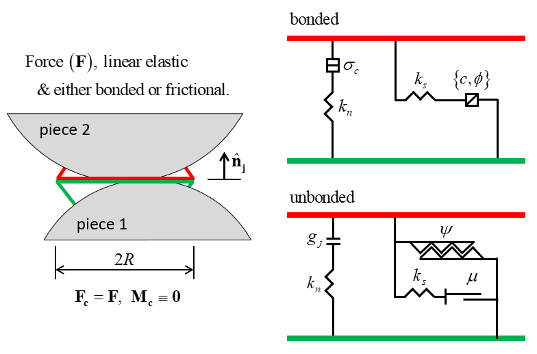
Figure 1: Behavior and rheological components of the smooth-joint model.
Activity-Deletion Criteria
If in small-strain mode (\(S_l = \rm false\)), a contact with the smooth-joint model is always active. In this mode, the contact will never be deleted. If in large-strain mode (\(S_l = \rm true\)), a contact with the smooth-joint model is active if the contact is bonded or if the contact gap is negative (i.e., the two pieces are overlapping).
Kinematic Variables
A typical smooth-joint contact is shown in Figure 2. The joint geometry consists of a planar interface separating two surfaces (denoted as surface 1 and surface 2). The interface orientation is defined by the unit-normal vector \({\bf \hat n_j}\), and surface 2 is defined such that \({\bf \hat n_j}\) points into surface 2. The unit normal is defined as:
where \(\theta_p\) is the dip angle and \(\theta_d\) the dip direction.
Joint orientation is fixed with respect to the global axes, and can only be changed by modifying the dip angle or dip direction. Whenever the joint orientation is changed (or is set initially), the two contacting entities (called piece 1 and piece 2) are associated with the appropriate joint surfaces. The contact unit-normal vector, \({\bf \hat n_c}\), is directed from the center of piece 1 to the center of piece 2. The dot product of \({\bf \hat n_c}\) and \({\bf \hat n_j}\) is used to determine in which surface each piece lies, such that piece 2 lies in surface 2 if and only if \({\bf \hat n_c \cdot \hat n_j} \geq 0\).
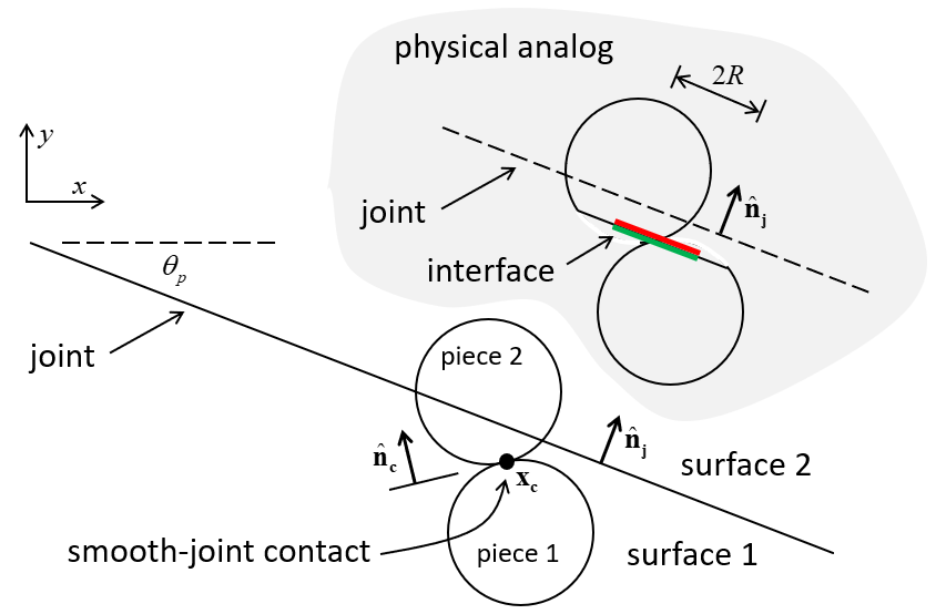
Figure 2: Joint and smooth-joint contact.
A smooth joint can be envisioned as a set of elastic springs uniformly distributed over a circular cross-section, centered at the contact point and oriented parallel with the joint plane. The area of the smooth-joint cross-section is given by:
where \(R^{(1)}\) and \(R^{(2)}\) are the piece radii.
Force-Displacement Law
As the smooth-joint orientation is not aligned with the contact normal, the relative displacement increment is resolved into joint normal and shear directions:
The accumulated normal and shear displacements are updated as:
The elastic portions of the normal (\(\Delta \stackrel{\frown}{{\delta_n}^e}\)) and shear (\(\Delta \stackrel{\frown}{{{\pmb δ}_\mathbf{s}}^e}\)) displacement increments are determined based on the value of the gap (\(g_i\) where \(g_i=0\) when the smooth joint is created). If bonded, then the entire displacement increment is elastic; if not bonded, then only the portion of the displacement increment that occurs while \(g_i<0\) is elastic.
The force-displacement law for the smooth-joint model updates the contact force:
where \(\mathbf{F}\) is the smooth-joint force. The force is resolved into normal and shear forces:
where \(F_n>0\) is tension.
The force-displacement law consists of the following steps (see Figure 3 and Figure 4):
Update the normal force:
(7)\[F_n = \left(F_n \right)_o + {k_n} A \Delta \stackrel{\frown}{{\delta_n}^e}\]where \(\left(F_n \right)_o\) is the smooth joint normal force at the beginning of the timestep and \(A\) is the bond cross-sectional area.
Calculate a trial shear force:
(8)\[\mathbf{F_{s}}^{*} =\left(\mathbf{F_{s}} \right)_{o} -k_{s} A \Delta \stackrel{\frown}{{\pmb{δ}_\mathbf{s}}^e}\]where \(\left(\mathbf{F_{s}} \right)_{o}\) is the shear force at the beginning of the timestep.
The frictional shear-strength limit is also computed:
(9)\[F_{s}^{\mu } =-\mu F_{n}.\]The forces, slip state, and bonding state are updated based on the bonding status.
If the smooth-joint model is unbonded (\(S_j<3\)), the shear force is updated:
(10)\[\begin{split}\mathbf{F_{s}} =\left\{\begin{array}{l} {\qquad \mathbf{F_{s}}^{*} ,\qquad \left\| \mathbf{F_{s}}^{*} \right\| \le F_{s}^{\mu } } \\ {\qquad F_{s}^{\mu } \left({\mathbf{F_{s}}^{*} \mathord{\left/ {\vphantom {\mathbf{F_{s}}^{*} \left\| F_{s}^{*} \right\| }} \right. } \left\| \mathbf{F_{s}}^{*} \right\| } \right),\qquad {\rm otherwise.}} \end{array}\right.\end{split}\]The slip state is updated:
(11)\[\begin{split}s=\left\{\begin{array}{l} {\qquad {\rm true},\qquad \left\| \mathbf{F_{s}} \right\| =F_{s}^{\mu } } \\ {\qquad {\rm false},\qquad {\rm otherwise.}} \end{array}\right.\end{split}\]If the slip state is true, then the contact is sliding. Whenever the slip states changes, the slip_change callback event occurs. While slipping, shear displacements produce an increase in normal force due to dilation:
(12)\[F_n = \left(F_n \right)_o + \left[ \stackrel{\frown}{{\delta_\mathbf{s}}^*} {\rm tan} \psi \right] {{k_n}} {{A}} = \left(F_n \right)_o + \left({{\left\| \mathbf{F_{s}}^{*} \right\| - F_{s}^{\mu }} \over {{k_s}}} \right) {k_n} {\rm tan} \psi\]where \(\mu\) is the friction coefficient and \(\psi\) is the dilation angle.
If the smooth-joint model is bonded (\(S_j=3\)), one updates the bonding status:
(13)\[\begin{split} S_j=\left\{\begin{array}{l} {\qquad 1,\qquad F_n \ge \sigma_c A \qquad (\rm{broken} \enspace \rm{in} \enspace \rm{tension})} \\ {\qquad 2, \qquad \left\| \mathbf{F_s}^* \right\| \ge \tau_c A \qquad (\rm{broken} \enspace \rm{in} \enspace \rm{shear})} \\ {\qquad 3, \qquad {\rm otherwise.}} \end{array}\right.\end{split}\]where \(\sigma_c\) is the bond normal strength and \(\tau_c\) is the bond shear strength (\(\tau_c = c - \left( {{F_n}} \over {{A}} \right){\rm tan} \phi\)). The following conditions are applied in each case:
If the bond has broken in tension (\(S_j=1\)), the normal and shear forces are reset:
(14)\[F_n = \left\| \mathbf{F_s} \right\| = 0.\]If the bond has broken in shear (\(S_j=2\)) and the bond is in tension, the normal and shear forces are reset as in Equation (14). If the bond is not in tension, the shear force is limited by Equation (10) but no dilation can occur. The slip state is updated as in Equation (11).
If the bond remains intact (\(S_j=3\)), the shear force is set to the trial shear force:
(15)\[\mathbf{F_s} = \mathbf{F_s}^*.\]
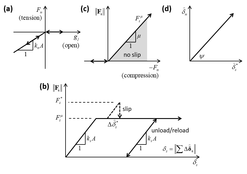
Figure 3: Force-displacement law for an unbonded joint: (a) normal force versus normal displacement; (b) shear force versus shear displacement; (c) strength envelope; and (d) normal displacement versus shear displacement during sliding.
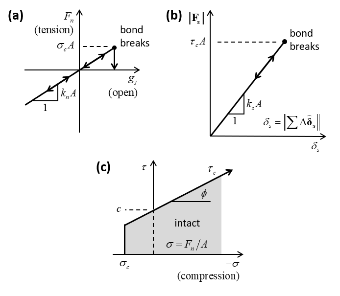
Figure 4: Force-displacement law for a bonded joint: (a) normal force versus normal displacement; (b) shear force versus shear displacement; and (c) strength envelope.
Energy Partitions
The smooth-joint model provides two energy partitions:
- strain energy, \(E_{k}\), stored in the linear springs; and
- slip energy, \(E_{\mu }\), defined as the total energy dissipated by frictional slip.
If energy tracking is activated, these energy partitions are updated as follows:
Update the strain energy:
(16)\[{\rm E} _{k} =\frac{1}{2} \left(\frac{\left(F_{n} \right)^{2} }{k_{n} } +\frac{\left\| \mathbf{F_{s}} \right\| ^{2} }{k_{s} } \right)\]Update the slip energy:
(17)\[\begin{split}\begin{array}{l} {E_{\mu } :=E_{\mu } +{\tfrac{1}{2}} \left(\left(\mathbf{F_{s}} \right)_{o} +\mathbf{F_{s}} \right)\cdot \Delta \pmb{δ} _\mathbf{s}^{\mu } } \\ [3mm] {{\rm with}\qquad \Delta \pmb{δ} _\mathbf{s}^{\mu } =\Delta \pmb{δ} _\mathbf{s} -\Delta \pmb{δ} _\mathbf{s}^{e} =\Delta \pmb{δ} _\mathbf{s} -\left(\frac{\mathbf{F_{s}} -\left(\mathbf{F_{s}} \right)_{o} }{k_{s} } \right)} \end{array}\end{split}\]where \(\left(\mathbf{F_{s}} \right)_{o}\) is the shear force at the beginning of the timestep, and the relative shear-displacement increment of this equation of the “Contact Resolution” section has been decomposed into an elastic \(\left(\Delta \pmb{δ} _\mathbf{s}^{e} \right)\) and a slip \(\left(\Delta \pmb{δ} _\mathbf{s}^{\mu } \right)\) component. The dot product of the slip component and the average shear force occurring during the timestep gives the increment of slip energy.
Additional information, including the keywords by which these partitions are referred to in commands and FISH, is provided in the table below.
| Name | Symbol | Description | Range | Accumulated |
|---|---|---|---|---|
energy‑strain |
\(E_{k}\) | Strain energy | \([0.0,+\infty)\) | NO |
energy‑slip |
\(E_{\mu}\) | Total energy dissipated by slip | \([0.0,+\infty)\) | YES |
Properties
The properties defined by the smooth-joint contact model are listed in the table below as a concise reference; see the “Contact Properties” section for a description of the information in the table columns. The mapping from the surface inheritable properties to the contact model properties is also discussed below.
| Keyword | Symbol | Description | Type | Range | Default | Modifiable | Inheritable |
|---|---|---|---|---|---|---|---|
| smoothjoint | Model name | ||||||
| sj_kn | \(k_n\) | Normal stiffness per unit area [force/volume] | FLT | \([0.0,+\infty)\) | 0.0 | YES | YES |
| sj_ks | \(k_s\) | Shear stiffness per unit area [force/volume] | FLT | \([0.0,+\infty)\) | 0.0 | YES | YES |
| sj_fric | \(\mu\) | Friction coefficient [-] | FLT | \([0.0,+\infty)\) | 0.0 | YES | YES |
| sj_da | \(\psi\) | Dilation angle [degrees] | FLT | \([0.0,+\infty)\) | 0.0 | YES | NO |
| sj_state | \(S_j\) | Joint bond state [-] | INT | {0;1;2;3} | 0 | YES | NO |
| \(\;\;\;\;\;\;\begin{cases} \mbox{0: unbonded} \\ \mbox{1: unbonded \& broke in tension} \\ \mbox{2: unbonded \& broke in shear} \\ \mbox{3: bonded} \end{cases}\) | |||||||
| sj_large | \(S_l\) | Large strain flag [-] | BOOL | {false,true} | false | YES | NO |
| sj_ten | \({\sigma}_c\) | Tensile strength [stress] | FLT | \([0.0,+\infty)\) | 0.0 | YES | NO |
| sj_coh | \(c\) | Cohesion | FLT | \([0.0,+\infty)\) | 0.0 | YES | NO |
| sj_fa | \(\phi\) | Joint friction angle [degrees] | FLT | \([0.0,+\infty)\) | 0.0 | YES | NO |
| sj_shear | \({\tau}_c\) | Shear strength [stress] | FLT | \([0.0,+\infty)\) | 0.0 | NO | NO |
| sj_rmul | \(\lambda\) | Joint radius multiplier [-] | FLT | \([0.0,+\infty)\) | 1.0 | YES | NO |
| sj_radius | \(R\) | Joint radius [length] | FLT | \([0.0,+\infty)\) | N/A | NO | N/A |
| sj_area | \(A\) | Joint area [surface] | FLT | \([0.0,+\infty)\) | N/A | NO | N/A |
| sj_slip | \(s\) | Slip state [-] | BOOL | {false,true} | false | NO | N/A |
| sj_gap | \(g_j\) | Joint gap [length] | FLT | \(\mathbb{R}\) | 0.0 | YES | NO |
| sj_unorm | \(\mathbf{\hat{n}_j}\) | Joint unit normal [force] | VEC | \(\mathbb{R}^3\) | \(\mathbf{0}\) | NO | NO |
| sj_un | \(\stackrel{\frown}{{\delta_n}}\) | Normal displacement [length] | FLT | \(\mathbb{R}\) | 0.0 | NO | N/A |
| sj_us | \(\stackrel{\frown}{{\pmb{δ}_\mathbf{s}}}\) | Shear displacement [length] | VEC | \(\mathbb{R}^3\) | \(\mathbf{0}\) | NO | N/A |
| dip | \(\theta_p\) | Joint dip [degrees] | FLT | [0.0,360.0] | 0.0 | YES | NO |
| ddir (3D) | \(\theta_d\) | Joint dip direction [degrees] | FLT | [0.0,180.0] | 0.0 | YES | NO |
| sj_fn | \(F_n\) | Normal force magnitude [force] | FLT | \(\mathbb{R}\) | 0.0 | YES | NO |
| sj_fs | \(\mathbf{F_s}\) | Shear force vector [force] | VEC | \(\mathbb{R}^3\) | \(\mathbf{0}\) | YES | NO |
Surface Property Inheritance
The linear stiffness per unit area, \(k_n\) and \(k_s\), and the friction coefficient, \(\mu\), may be inherited from the contacting pieces. Remember that for a property to be inherited, the inheritance flag for this property must be set to true, and both contacting pieces must hold a property with this name.
The stiffness are inherited assuming that both pieces’ stiffness act in series:
where (1) and (2) denote the properties of piece 1 and 2, respectively. The friction coefficient is inherited using the minimum friction coefficient:
Methods
| Method | Arguments | Symbol | Type | Range | Default | Description |
|---|---|---|---|---|---|---|
| sj_setforce | N/A | Set the force | ||||
| bond | Bond the joint if \(g_j \in G\) | |||||
| gap | \(\mathbb{G}\) | VEC2 | \(\mathbb{R}^2\) | \((-\infty,0]\) | Gap interval | |
| unbond | Unbond the joint if \(g_j \in G\) | |||||
| gap | \(G\) | VEC2 | \(\mathbb{R}^2\) | \((-\infty,0]\) | Gap interval | |
sj_setforce
Set the smooth-joint normal force (\(F_n\)) from the current contact force:
Bond
Create a smooth-joint bond (\(S_j=3\)) by bonding the interface if the contact gap between
the pieces is within the bonding-gap interval. If no gap is specified, then the contact is
bonded if the pieces overlap. A single value can be specified with the gap keyword corresponding to the maximum gap.
One can ensure the existence of contacts
between all pieces with a contact gap less than a specified bonding gap (\(g_{b}\)) by
specifying \(g_{b}\) as the proximity in the contact cmat default command of the
Contact Model Assignment Table (CMAT).
Unbond
Remove a smooth-joint bond by unbonding (\(S_j=0\)) the interface if the contact gap between the pieces is within the bonding-gap interval. If no gap is specified, then the contact is unbonded if the pieces overlap. A single value can be specified with the gap keyword corresponding to the maximum gap. If the interface becomes unbonded, then the bond state becomes unbonded. The smooth-joint force is unaffected and will be updated during the next cycle.
Callback Events
| Event | Array slot | Value Type | Range | Description |
|---|---|---|---|---|
| contact_activated | Contact becomes active | |||
| 1 | C_PNT | N/A | Contact pointer | |
| slip_change | Slip state has changed | |||
| 1 | C_PNT | N/A | Contact pointer | |
| 2 | INT | {0;1} | Slip change mode | |
| {0;1} | \(\;\;\;\;\;\;\begin{cases} \mbox{0: slip has initiated} \\ \mbox{1: slip has ended} \end{cases}\) | |||
| bond_break | Bond has broken | |||
| 1 | C_PNT | N/A | Contact pointer | |
| 2 | INT | {1;2} | Failure mode | |
| \(\;\;\;\;\;\;\begin{cases} \mbox{1: failed in tension} \\ \mbox{2: failed in shear} \end{cases}\) | ||||
| 3 | FLT | \([0.0,+\infty)\) | Failure strength [stress] (tension or shear, according to the failure mode) | |
Usage and Verification Examples
The smooth-joint contact model is demonstrated in the “Slip on a Fault” tutorial.
| Was this helpful? ... | FLAC3D © 2019, Itasca | Updated: Feb 25, 2024 |